Skip to main content
Data is the key power source of today’s software solutions. But having to handle too much data can become a challenge, affecting your project’s requirements for talents, equipment, and financial and computational resources.
Artificial intelligence (AI) technologies offer a solution to the problem of limited data storage capacity in the form of data compression. In this article, we discuss different types of unsupervised deep learning models you can use to reduce the size of your data. We also provide a practical example of how to compress data using deep learning neural networks called autoencoders to reduce image file sizes.
This article will be useful for development teams looking to reduce the required data storage capacity of their projects.
Contents:
Core data compression algorithms: lossy vs lossless
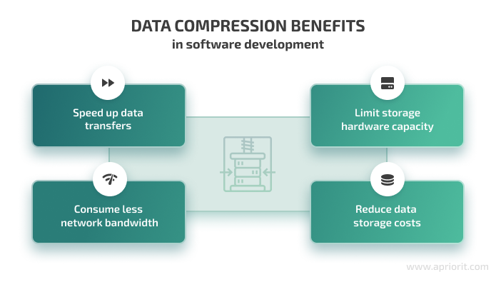
There are two major concerns related to data storage capacity limitations:
- Data storage capacity cost — Storing and processing more data requires deploying additional data centers, which leads to increased data storage costs.
- Data center maintenance and scaling — Deploying additional data centers also requires allocating additional resources for their configuration and maintenance.
Compressing your data can help you effectively address these concerns and overcome the challenge of limited storage capacity.
Data compression is the process of encoding, restructuring, or modifying data in order to reduce its size. As a result of data compression, you receive re-encoded information that takes up less storage space.
Compressing your data comes in handy when you need to:
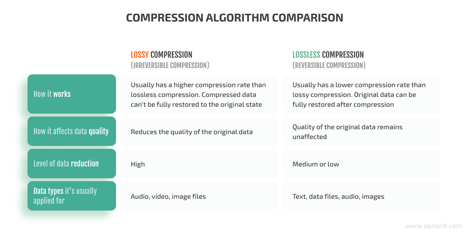
Existing data compression algorithms can be divided into two large classes:
- Lossy algorithms are commonly used to compress images and audio. These algorithms allow for achieving high compression ratios with a selective loss of quality. However, by definition, it’s impossible to fully recover the original data after lossy compression.
- Lossless algorithms reduce data size in a way that allows for full restoration of the original data from a compressed file. These algorithms are mostly used in communication systems and data archivers. Some lossless algorithms are also used for compressing audio and graphics information.
In general, we can outline four main types of data that may be compressed using these algorithms:
- Audio — For audio compression, algorithms are implemented as audio codecs — programs that can compress and decompress audio files. Depending on the task at hand and the original file format, you can choose codecs that use either lossy or lossless algorithms. For instance, MP3 is the most ubiquitous lossy codec, while FLAC is a major lossless codec.
- Images — Digitally stored images can be compressed to reduce the size of the original image and therefore save storage space and cut down the time needed to transfer the image over the network. Similar to audio files, images can be compressed using either lossy or lossless algorithms. The most popular lossy algorithm is JPEG, and widely used lossless algorithms are GIF and PNG.
- Video — Video compression is a combination of image compression and audio compression. Because of the high data rate required for uncompressed video, most video files are compressed using lossy compression. The most prevalent form of lossy video compression is MPEG.
- Text — Text data is usually compressed using lossless algorithms that find repeated sequences in the text and replace them with shorter representations. One of the commonly used lossless text compression formats is GZIP.
One way to efficiently apply these data compression algorithms is by using them as part of a dedicated deep learning (DL) neural network. Later in this article, we’ll take a look at two practical examples of image compression using deep learning models. But first, let’s go over some basic terms.
Need help automating data size reduction?
Ensure efficient image processing to optimize data storage and improve your solution’s performance by leveraging the expertise of Apriorit’s AI and Python engineers.
The role of neural networks in data compression
Deep learning aims to solve real-world problems using neural networks that can, to some extent, mimic the way the human brain processes information and makes decisions. A neural network consist of multiple neurons that are usually arranged in three layers:
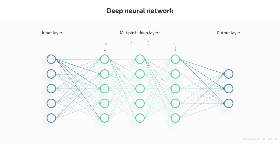
- The input layer is analogous to dendrites — nerve cell extensions responsible for receiving signals from other cells in the human brain. This layer brings the data you feed to your neural network into the system, where it will be processed by deeper layers of artificial neurons.
- The hidden layer is comparable to the body of a human brain’s neuron and sits between the input layer and output layer (which is akin to the synaptic outputs in the brain). This is where the majority of data processing takes place. Neural networks with multiple hidden layers are called deep neural networks.
- The output layer is the final layer of a neural network. Using a transfer function, the system sends the output generated by the weighted inputs to the outcome layer, thus producing outcome variables.
There are also two ways you can train your deep learning models:
- Supervised learning, where a set of examples — the training set — is submitted as input to the system during the training phase. Each input is labeled with a desired output value so that the system can detect underlying patterns relating inputs to outputs, then use these patterns to produce accurate outcomes when processing new data.
- Unsupervised learning, where the neural network is supposed to examine the underlying structure of the data and search for common characteristics or patterns in it to produce an outcome. In contrast to supervised learning, there are no correct outputs.
In some cases, you might use a mix of labeled and unlabeled data to train your neural network, thus applying what is called semi-supervised learning.
When compared to non-AI data compression methods, the use of neural networks allows for:
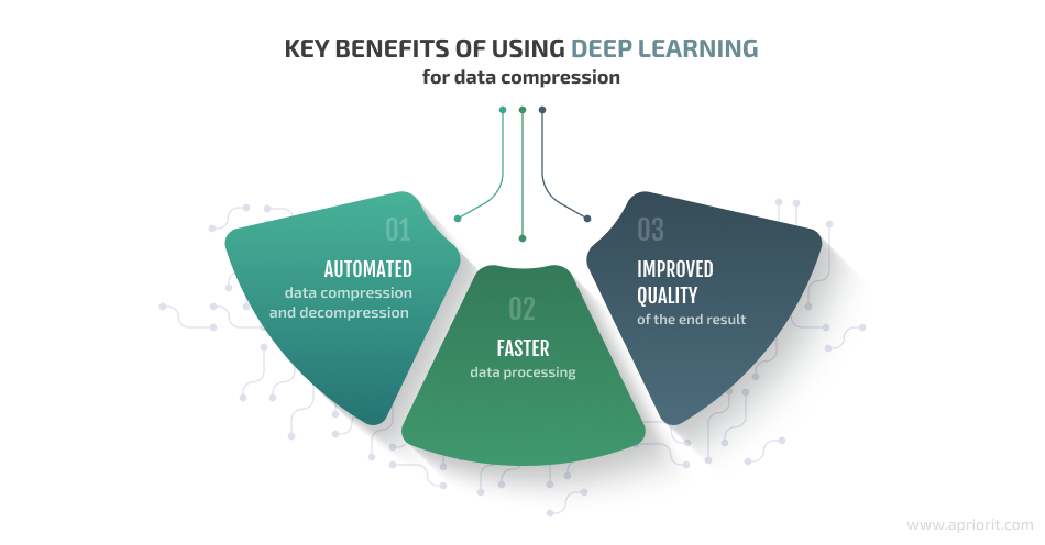
- Automating data compression and decompression
- Increasing the speed of data processing
- Improving the quality of the end result
Depending on the format of the original file and the task at hand, you may compress data using different neural networks: long short-term memory, a recurrent neural network, or autoencoders.
In this article, we focus on image compression using autoencoders, discussing in detail how to save the most possible storage space using lossy data compression methods with deep learning and analyzing a practical example of such an operation.
Read also
Leverage AI to transform your image processing capabilities.
Explore how artificial intelligence is revolutionizing image processing, from improving quality to automating complex tasks. Read the full article from Apriroit experts for more insights, technologies, and ways to overcome common challenges.

Using autoencoders for data compression: practical examples
Imagine trying to remember a large number. You’ll probably start by looking for a pattern that’s easy to remember and that will help you reconstruct the entire sequence later. That’s pretty much how an autoencoder neural network works.
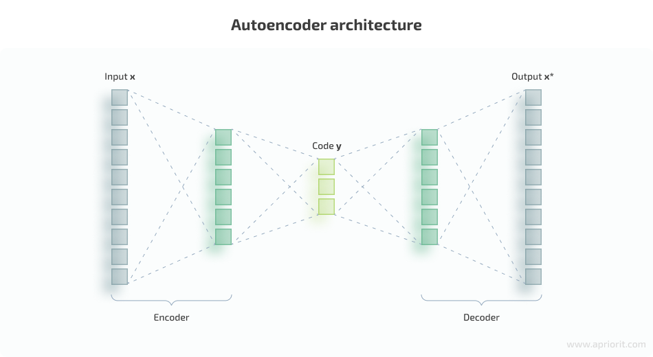
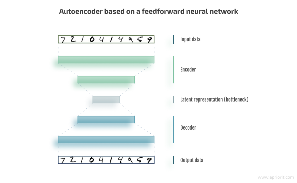
Basic autoencoders are feedforward neural networks that reconstruct the input signal from the output. An autoencoder consists of three parts:
- An encoder layer that compresses — encodes — the input into a latent space representation with a reduced dimension.
- Code that represents the compressed input that is fed to the next layer.
- A decoder layer that decodes the encoded data back to its original dimension. The decoded file is a lossy reconstruction of the original data and is reconstructed from the latent space representation.
Complex autoencoders can be based on a convolutional neural network (CNN) and are usually called convolutional autoencoders. We’ll get back to working with such networks later in this article.
Now, let’s see how an autoencoder works in detail:
An encoder layer maps the input x to a lower-dimensional feature vector y, and then a decoder layer reconstructs the input x* from y. However, autoencoders are designed in such a way that they can’t exactly copy the input to the output: they have a special low-dimension layer inside that is considered to be an encoding of the input signal.
The input signal is restored with errors due to coding losses, but in order to minimize them, the neural network has to learn to select the most important features. So we train the neural network by comparing x to x* and optimizing the parameters to increase the similarity between x and x*.
Below, you can see what an autoencoder architecture looks like:
Autoencoders learn automatically from data examples you feed to the neural network, so it’s easy to train specialized instances of the algorithm that will perform well on a certain type of input data. But being data-specific, they can only compress data similar to what they have been trained on.
This peculiarity makes autoencoders mostly impractical for real-world data compression problems: you can only use them on data that’s similar to what they were trained on, and making a more generalized autoencoder would require training it on several types of data. However, if you only work with a certain type of well-structured data and some quality losses are acceptable, you can use autoencoders to solve the problem of limited data storage capacity.
Now that we’ve grasped the core idea of the way autoencoders work and where you can use them, let’s move to a practical example of working with some. In the following sections, we provide examples of image compression with deep learning, both using the Keras framework written in Python but with two different neural networks.
Related project
Building an AI-based Healthcare Solution
Discover how Apriorit helped a client create a cutting-edge AI-based system for healthcare, saving doctors’ time and achieving 90% precision and a 97% recall rate detecting and measuring follicles.

Example 1: Simple image compression with Keras
Let’s start with a rather simple task and try performing image compression in Keras by compressing black-and-white images with a basic autoencoder. For this case, an autoencoder based on a typical feedforward neural network will be enough.
As the data source for our model, we chose the public MNIST dataset that contains handwritten digits commonly used for training various image processing systems:
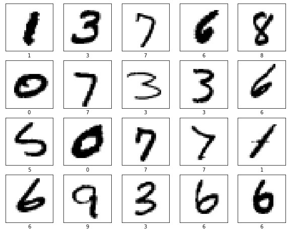
Image 1: Example of handwritten digits from the MNIST dataset
Let’s start our practical experiment.
1. First, we install some libraries with the help of the pip package installer:
pip install tensorflow==2.4.3
pip install keras==2.4.3
pip install matplotlib==3.3.4
pip install numpy==1.19.5
pip install extra-keras-datasets==1.2.02. Then we move to writing a simple deep learning model and import required classes and modules:
from keras.layers import Input, Dense
from keras.datasets import mnist
from keras.models import Model

import numpy as np3. Now, let’s write a function that creates a simple autoencoder with one hidden layer of 64 neurons for the encoder and decoder parts of the model:
IMAGE_SIZE = 784 # 28 * 28 pixels

def encoder(input_image, code_dimention):
    layer1 = Dense(64, activation='relu')(input_image)
    layer2 = Dense(code_dimention, activation='sigmoid')(layer1)

    return layer2

def decoder(encoded_image):
    layer1 = Dense(64, activation='relu')(encoded_image)
    layer2 = Dense(IMAGE_SIZE, activation='sigmoid')(layer1)

return layer24. Next, we load the dataset and start training the neural network. In the example below, we’re using 10 epochs (meaning that we run the entire dataset through the network ten times back and forth) with a batch size of 64:
input_image = Input(shape=(IMAGE_SIZE, ))

model = Model(input_image, decoder(encoder(input_image, 100)))
model.compile(loss='mean_squared_error', optimizer='nadam')

(x_train, _), (x_test, _) = mnist.load_data()

# Normalize data
x_train = x_train.astype('float32') /= 255.0
x_train = x_train.reshape((len(x_train), np.prod(x_train.shape[1:])))

x_test = x_test.astype('float32') /= 255.0
x_test = x_test.reshape((len(x_test), np.prod(x_test.shape[1:])))

# Training
model.fit(x_train, x_train, batch_size=64, epochs=10, validation_data=(x_test, x_test), shuffle=True)Decompression results will differ depending on the chosen code size — the number of nodes in the code layer.
For example, this is what the result of AI-based image compression and decompression looks like with code size = 128:
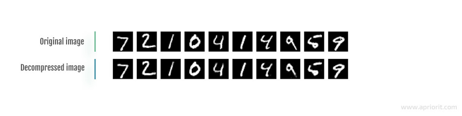
Image 2: Image compression and decompression with code size = 128
If we compress and decompress the same image with code size = 32, this is what the result looks like:
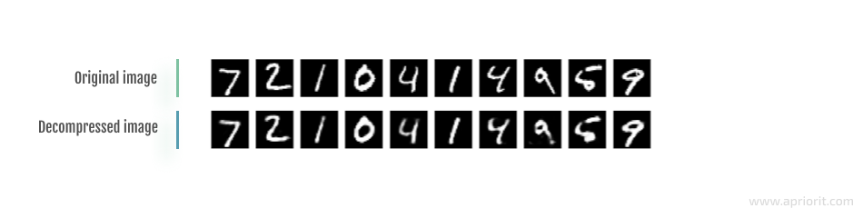
Image 3: Image compression and decompression with code size = 32
And if we reduce the code size even more and try compressing and decompressing that image with code size = 8, the result would look like this:
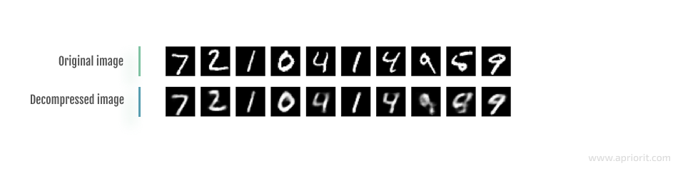
Image 4: Image compression and decompression with code size = 8
As you can see, the quality of decompressed data gets worse as you reduce the code size. This is why it’s important to properly determine a reasonable code dimension (the extent to which the data will be compressed) for a particular task at hand in order to maintain a tolerable level of data quality after decompression.
In this example, we were able to compress the original images almost a hundred times without facing any significant quality losses.
Now, let’s get to a bit more challenging scenario of using autoencoders in Keras for image compression.
Read also
Applying Deep Learning to Classify Skin Cancer Types
Learn how using deep learning can help automate and improve the accuracy of skin cancer detection and diagnosis. Apriorit experts show a practical example of creating such a solution, as well as offer a way to overcome the challenge of a lack of data for network training.
Example 2: Advanced image compression with Keras
Compressing small black-and-white images is a rather trivial task. Let’s try something more difficult, this time using the same framework but with a different dataset and a different neural network.
As for our data source, let’s use the STL-10 dataset, which has ten different classes of colored images:
- Airplane
- Bird
- Car
- Cat
- Deer
- Dog
- Horse
- Monkey
- Ship
- Truck
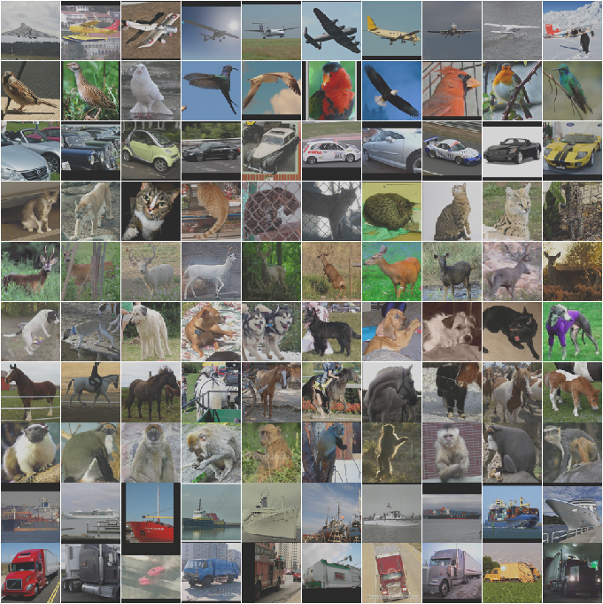
Image 5: Examples of STL-10 dataset contents
The network we used in the previous section was simple and can only handle black-and-white numbers. It’s not suitable for handling different classes of colored images. To be able to compress and then decompress such a dataset, we need a more complex deep neural network architecture based on a convolutional neural network.
CNNs were specially designed for processing images. They have multiple special convolutional layers that can spot features in different parts of an image. A typical architecture of a CNN-based autoencoder looks like this:
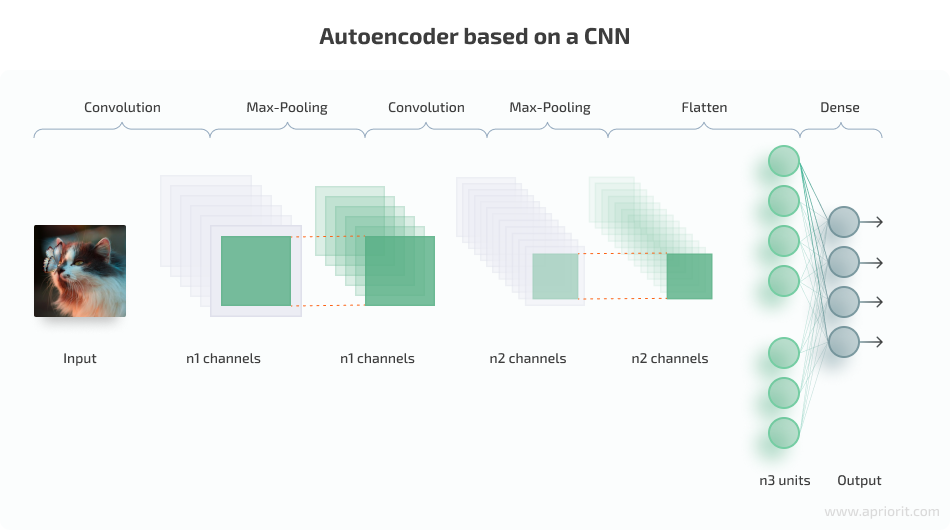
Image 6: Autoencoder based on a CNN. Image Credit: Jose Alberto Benítez Andrades
To compress images from the STL-10 dataset, we once again will use the Keras framework.
1. Start with importing required classes and modules:
from keras.layers import Input, Conv2D, MaxPooling2D, UpSampling2D, BatchNormalization, Activation, Dropout, Flatten
from keras.models import Model
from extra_keras_datasets import stl10

import numpy as np2. Next, define a convolutional architecture with eight convolutional and three max-pooling layers for the encoder.
def encoder(input_image):
    conv1 = Conv2D(32, (3, 3), activation='relu', padding='same')(input_image) #96 x 96 x 32
    conv1 = BatchNormalization()(conv1)
    conv1 = Conv2D(32, (3, 3), activation='relu', padding='same')(conv1) #96 x 96 x 32
    conv1 = BatchNormalization()(conv1)
    conv1 = Conv2D(32, (3, 3), activation='relu', padding='same')(conv1) #96 x 96 x 32
    conv1 = BatchNormalization()(conv1)
    conv1 = Conv2D(32, (3, 3), activation='relu', padding='same')(conv1) #96 x 96 x 32
    conv1 = BatchNormalization()(conv1)
    conv1 = MaxPooling2D(pool_size=(2, 2))(conv1) #48 x 48 x 32
    conv1 = Dropout(0.4)(conv1)

    conv2 = Conv2D(64, (3, 3), activation='relu', padding='same')(conv1) #48 x 48 x 64
    conv2 = BatchNormalization()(conv2)
    conv2 = Conv2D(64, (3, 3), activation='relu', padding='same')(conv2) #48 x 48 x 64
    conv2 = BatchNormalization()(conv2)
    conv2 = Conv2D(64, (3, 3), activation='relu', padding='same')(conv2) #48 x 48 x 64
    conv2 = BatchNormalization()(conv2)
    conv2 = Conv2D(64, (3, 3), activation='relu', padding='same')(conv2) #48 x 48 x 64
    conv2 = BatchNormalization()(conv2)
    conv2 = MaxPooling2D(pool_size=(2, 2))(conv2) #24 x 24 x 64
    conv2 = Dropout(0.4)(conv2)

    conv3 = Conv2D(64, (3, 3), activation='relu', padding='same')(conv3) #24 x 24 x 64
    conv3 = BatchNormalization()(conv3)
    conv3 = Conv2D(64, (3, 3), activation='relu', padding='same')(conv3) #24 x 24 x 64
    conv3 = BatchNormalization()(conv3)
    conv3 = Conv2D(64, (3, 3), activation='relu', padding='same')(conv3) #24 x 24 x 64
    conv3 = BatchNormalization()(conv3)
    conv3 = Conv2D(64, (3, 3), activation='relu', padding='same')(conv3) #24 x 24 x 64
    conv3 = BatchNormalization()(conv3)
    conv3 = MaxPooling2D(pool_size=(2, 2))(conv3) #12 x 12 x 64
    conv3 = Dropout(0.4)(conv3)

    conv4 = Conv2D(32, (3, 3), activation='relu', padding='same')(conv3) #12 x 12 x 32
    conv4 = BatchNormalization()(conv4)
    conv4 = Conv2D(32, (3, 3), activation='relu', padding='same')(conv4) #12 x 12 x 32
    conv4 = BatchNormalization()(conv4)
    conv4 = Conv2D(32, (3, 3), activation='relu', padding='same')(conv4) #12 x 12 x 32
    conv4 = BatchNormalization()(conv4)
    conv4 = Conv2D(32, (3, 3), activation='relu', padding='same')(conv4) #12 x 12 x 32

    encoded = BatchNormalization()(conv4)

    return encoded

def decoder(encoded_image):
    conv5 = Conv2D(32, (3, 3), activation='relu', padding='same')(conv4) #12 x 12 x 32
    conv5 = BatchNormalization()(conv5)
    conv5 = Conv2D(32, (3, 3), activation='relu', padding='same')(conv5) #12 x 12 x 32
    conv5 = BatchNormalization()(conv5)
    conv5 = Conv2D(32, (3, 3), activation='relu', padding='same')(conv5) #12 x 12 x 32
    conv5 = BatchNormalization()(conv5)
    conv5 = Conv2D(32, (3, 3), activation='relu', padding='same')(conv5) #12 x 12 x 32
    conv5 = BatchNormalization()(conv5)
    conv5 = UpSampling2D((2,2))(conv5) #24 x 24 x 32

    conv6 = Conv2D(64, (3, 3), activation='relu', padding='same')(conv5) #24 x 24 x 64
    conv6 = BatchNormalization()(conv6)
    conv6 = Conv2D(64, (3, 3), activation='relu', padding='same')(conv6) #24 x 24 x 64
    conv6 = BatchNormalization()(conv6)
    conv6 = Conv2D(64, (3, 3), activation='relu', padding='same')(conv6) #24 x 24 x 64
    conv6 = BatchNormalization()(conv6)
    conv6 = Conv2D(64, (3, 3), activation='relu', padding='same')(conv6) #24 x 24 x 64
    conv6 = BatchNormalization()(conv6)
    conv6 = UpSampling2D((2,2))(conv6) #48 x 48 x 64

    conv7 = Conv2D(64, (3, 3), activation='relu', padding='same')(conv6) #48 x 48 x 64
    conv7 = BatchNormalization()(conv7)
    conv7 = Conv2D(64, (3, 3), activation='relu', padding='same')(conv7) #48 x 48 x 64
    conv7 = BatchNormalization()(conv7)
    conv7 = Conv2D(64, (3, 3), activation='relu', padding='same')(conv7) #48 x 48 x 64
    conv7 = BatchNormalization()(conv7)
    conv7 = Conv2D(64, (3, 3), activation='relu', padding='same')(conv7) #48 x 48 x 64
    conv7 = BatchNormalization()(conv7)
    conv7 = UpSampling2D((2,2))(conv7) #96 x 96 x 64

    conv8 = Conv2D(32, (3, 3), activation='relu', padding='same')(conv7) #96 x 96 x 32
    conv8 = BatchNormalization()(conv8)
    conv8 = Conv2D(32, (3, 3), activation='relu', padding='same')(conv8) #96 x 96 x 32
    conv8 = BatchNormalization()(conv8)
    conv8 = Conv2D(32, (3, 3), activation='relu', padding='same')(conv8) #96 x 96 x 32
    conv8 = BatchNormalization()(conv8)
    conv8 = Conv2D(32, (3, 3), activation='relu', padding='same')(conv8) #96 x 96 x 32
    conv8 = BatchNormalization()(conv8)

return Conv2D(3, (3, 3), activation='sigmoid', padding='same')(conv8) #96 x 96 x 3In our case, the encoder takes 27,648 numbers as input (96 width * 96 height * 3 RGB) and produces 4,608 numbers as the output — that’s the encoding of the initial image.
3. Now, load the dataset and start training your model (100 epochs with batch size 32):
input_image = Input(shape=(96, 96, 3))

model = Model(input_image , decoder(encoder(input_image)))
model.compile(loss='mean_squared_error', optimizer='nadam')

(x_train, _), (x_test, _) = stl10.load_data()

# Normalize data
x_train = x_train.astype('float32') /= 255.0
x_test = x_test.astype('float32') /= 255.0

# Training
model.fit(x_train, x_train, batch_size=32, epochs=100, validation_data=(x_test, x_test), shuffle=True)Here’s the result we get after compressing this dataset six times:
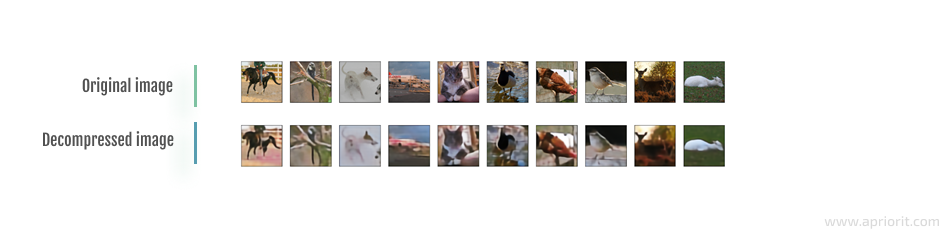
Image 7: Example of a compressed image from the STL-10 dataset
As you can see, there’s a noticeable difference in quality between the original image and its decompressed version. For this example, we used a rather simple neural network that you can train properly even when your computational power is limited to your CPU only.
Depending on the task at hand, you might have different requirements for the quality of data after decompression. To increase the quality of decoded images while still providing some data size reduction, you will need to use an autoencoder with a much more complex architecture that requires GPU resources for training and apply some fine-tuning techniques during the process. Such an autoencoder would be even better at extracting important features from the processed data so the original image would be restored with fewer quality losses. The stricter your requirements for the quality of decoded data, the more complex the deep neural network and the more rounds of training you need.
Conclusion
Modern software requires processing, storing, and transferring tons of data on a daily basis. Yet network bandwidth and storage capacity remain limitations for most data-driven products and services.
To effectively solve the problem of limited data storage capacity, you can use dedicated AI-powered solutions called autoencoders.
Depending on your data quality requirements, you can choose autoencoders based on more simple or more complex deep neural networks and adjust the number of trainings your model goes through. In some cases, you might also need to apply additional noise reduction algorithms and fine-tuning techniques to improve the quality of the decompressed output.
As autoencoders are data-specific, they’re more suitable for solutions that work with well-structured data and allow for reasonable quality losses after decompression. If your solution has strict data quality requirements or works with multiple types of data, Apriorit’s AI experts will gladly help you choose a more efficient approach to data compression using deep learning methods.
Looking for experienced AI developers?
Delegate the configuration and training of your AI models to Apriorit experts to ensure high efficiency, flawless performance, and great security for your software!
Have a question?
Ask our expert!
R&D Delivery Manager