Applying Deep Learning to Classify Skin Cancer Types

More and more developers are considering applying deep learning to real-world problems. Deep learning has skyrocketed in popularity in recent years, solving issues in various fields including medicine. In particular, neural networks can be used to classify types of skin lesions. These networks are trained on medical datasets and continually learn.

Despite constant improvements in medicine and quality of life, skin cancer remains an issue. According to statistics by the Skin Cancer Foundation, one in five Americans will develop skin cancer by age 70.

When it comes to skin cancer, time is an enemy: the earlier doctors detect it, the better. Modern magnification techniques allow specialists to conduct a detailed examination of suspicious skin lesions before proceeding to the next steps, such as biopsy, to make a precise diagnosis. Still, there’s no guarantee that a doctor’s diagnosis is accurate.

In this article, we explain how AI can enhance current diagnostic technologies, list major challenges on the way, and approach the problem of classifying seven types of skin cancer lesions using deep learning. This article will be helpful for those considering applying deep learning for healthcare applications.

Using deep learning for medical diagnosis: benefits and challenges

Deep learning — in the form of image classification and semantic segmentation — is being used to solve various problems with computer vision. Deep learning algorithms demonstrate astonishingly accurate results (greater than 95% accuracy) when it comes to classifying cats and dogs or everyday objects like cars and chairs.

The reason for these great results is that a lot of huge datasets (Pascal VOC 2007, ImageNet, COCO) have already been designed — by compiling freely available images of pets and everyday objects — to help neural networks learn how to classify these things.

Medicine is one of the most important fields where AI can be applied. AI technologies in healthcare can solve various issues related to diagnosis and detection by:

• Processing gigabytes of images and data in a short amount of time
• Constantly training and learning to improve the accuracy of its results
• Exceeding a human’s reading capacity
• Detecting patterns and details better than the naked human eye
• Speeding up diagnosis and treatment
• Enabling precision medicine, whereby doctors use genetic changes in a patient’s tumor to determine an adequate treatment plan
• Eliminating the subjective judgment of individual physicians

Deep learning technologies are perfect for classifying various types of skin cancer while they can distinguish specific graphic patterns of skin lesions. We examined the difference between machine learning and deep learning in our previous article. However, developers still need to overcome several challenges in order to create flawless applications.

To accomplish a complicated task like detecting and fighting diseases, a deep learning model needs to be trained on thousands of samples. Unfortunately, developers often don’t have enough images to properly train neural networks. Therefore, tasks such as detecting and fighting diseases are usually performed in conditions of severe lack of data, time, and computational power.

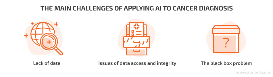
Lack of data — Deep learning requires large amounts of data to train neural networks and constantly improve the accuracy of their results. Unfortunately, it’s not that easy to find a ready-to-go database with thousands of precisely the images you need, especially for less prevalent diseases. And gathering data manually is often not an option, as it can take too much time. To overcome this issue, developers may use tools that slightly alter existing images in a training set in order to provide more data for training. In the best-case scenario, medical institutions will gather more images and data for future datasets.

Issues of data access and integrity — Medical data is often siloed or slightly obfuscated by healthcare providers in order to protect patient health information, guard against medical malpractice claims, and compete with other medical institutions. Another issue is the lack of infrastructure to share data between hospitals, clinics, institutions, and other healthcare establishments.

The black box problem — Learning by itself, AI often comes up with conclusions that humans have never thought of and sometimes can’t even comprehend. Complex approaches to machine learning make the machine’s automated decision-making processes inscrutable, which means that users receive results without understanding how the system arrived at them. Therefore, doctors can consider it dangerous to rely on decisions made by AI. Developers are still working on solving the black box problem.

Despite all the challenges, various medical solutions already use AI to successfully enhance organizational and treatment processes. Here are a few of them:

• Nuance assists in administrative workflow automation, providing real-time clinical documentation guidance and ensuring consistent recommendations.
• AI-assisted robotic surgery reduces inefficiencies of surgical attendants and improves outcomes. AI systems gather and process tons of data to help surgeons better understand which techniques result in better outcomes.
• Healthcare applications can gather data about heart rate, calories burned, kilometers walked, etc. An AI system can then analyze this information and suggest lifestyle improvements. This data can also be shared with doctors to provide them with more data on a patient’s habits.

Now that we’ve highlighted major benefits of AI and listed the main challenges of using deep learning in medicine, let’s move further. To create a network that can classify seven types of skin cancer, we have to prepare the environment, find a dataset, train our network, and check its performance.

Preparing the environment

To apply deep learning for skin cancer detection, we first have to prepare the environment for our network. Training a deep learning model requires significant resources: tens or even hundreds of gigabytes of disk space, lots of RAM, and a decent GPU. To meet all these requirements, we use Google Colaboratory (also known as Colab), which provides us an instance of Ubuntu 18 with 300GB of disk space and an accessible file system, 12 GB of RAM, and 12GB of Nvidia K80 GPU memory that can be used up to 12 hours continuously.

During our research, we found a way to obtain twice as much RAM as usual in Google Colaboratory. All you need to do is crash the current environment with an out of memory error (simply start loading all of your data until you run out of memory) and you’ll be offered increased RAM. Although this trick works for now, it’s likely to be disabled in the near future.

 

Figure 1. Colab environment configuration after accepting the offer of increased RAM

Since the Colab instance lasts up to 12 hours and training processes may take a lot of time, we need to optimize our use of the environment. There are three basic steps to optimize this task:

1) Load your data to Google Drive.

2) Mount your Google Drive to Google Colab.

 

Figure 2. Mounting Google Drive in Google Colaboratory

Once you click the Mount Drive button, the following block of code will appear:

from google.colab import drive
drive.mount('/content/drive')

3) Copy all your data to the Colaboratory file system.

Note: Uploading your data to Colab from the local system will take a lot of time. However, you can accelerate the process of copying files to Colab from Google Drive with one command:

# Copy files from Google Drive to the VM local filesystem
!cp -r "/content/drive/My Drive/skin-cancer-mnist-ham10000" ./skin-cancer-mnist-ham10000

Then import all the modules you’ll use for the task:

import os
import shutil
import pandas as pd
import numpy as np
import matplotlib.pyplot as plt
from sklearn.model_selection import train_test_split
from tensorflow.keras.layers import Dense, Dropout, GlobalAveragePooling2D
from tensorflow.keras.optimizers import Adam
from tensorflow.keras.metrics import categorical_crossentropy
from tensorflow.keras.preprocessing.image import ImageDataGenerator
from tensorflow.keras.models import Model
from tensorflow.keras.callbacks import EarlyStopping, ModelCheckpoint
from tensorflow.keras.applications.resnet import ResNet152, preprocess_input
%matplotlib inline

Now that we’ve optimized the Colab environment, let’s move on to datasets.

Working with datasets

Machine learning for cancer detection isn’t possible without data. Unfortunately, there are very few ready-to-use datasets for training a neural network to classify skin lesions. However, we managed to find the HAM10000 dataset, which is a decent dataset that contains a large collection of multi-source dermatoscopic images of common pigmented skin lesions.

The HAM10000 dataset consists of 10,000 images of seven classes of skin cancer. As with any dataset, it may contain errors and duplicates. Therefore, we have to preprocess this data first.

After we’ve finished copying the folder with the HAM10000 dataset, we can find it in our Colab VM filesystem.

 

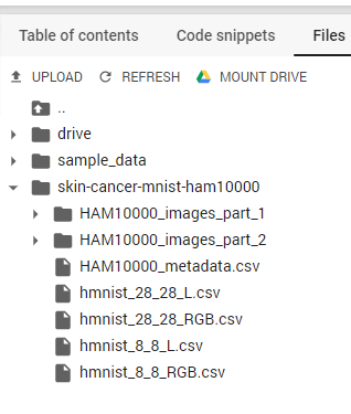
Figure 3. The HAM10000 dataset in the Colab VM filesystem

Now we can see that all images in the dataset are located in two folders and are labeled as .csv files. Let’s simplify things by creating the following directory structure:

 

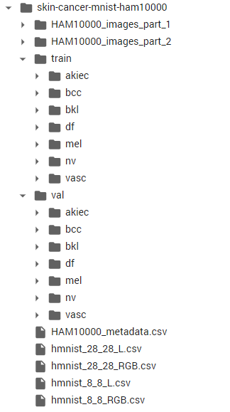
Figure 4. Simplified directory

To create this directory structure, we used this code:

import os
train_dir = 'train'
os.mkdir(train_dir)
val_dir = 'val'
os.mkdir(val_dir)
os.mkdir(os.path.join(train_dir, 'nv'))
os.mkdir(os.path.join(train_dir, 'mel'))
os.mkdir(os.path.join(train_dir, 'bkl'))
os.mkdir(os.path.join(train_dir, 'bcc'))
os.mkdir(os.path.join(train_dir, 'akiec'))
os.mkdir(os.path.join(train_dir, 'vasc'))
os.mkdir(os.path.join(train_dir, 'df'))
os.mkdir(os.path.join(val_dir, 'nv'))
os.mkdir(os.path.join(val_dir, 'mel'))
os.mkdir(os.path.join(val_dir, 'bkl'))
os.mkdir(os.path.join(val_dir, 'bcc'))
os.mkdir(os.path.join(val_dir, 'akiec'))
os.mkdir(os.path.join(val_dir, 'vasc'))
os.mkdir(os.path.join(val_dir, 'df'))

Now we have train and val directories that contain images for each class of skin cancer for training and validation purposes, respectively.

Let’s take a look at the metadata. To read and work with metadata, we use the Pandas Python Data Analysis Library. We import the file with the dataset into Pandas and use the head command to display the first five records in the form of a table.

import pandas as pd
df_data = pd.read_csv('HAM10000_metadata.csv')
df_data.head()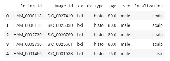

 

Figure 5. Pandas Python data analysis library

In the table above, the dx column corresponds to the class of the cancer. To train the neural network and make sure that it’s learning, we need to split our training data into training and validation subsets. The training portion of the data will only be used for training, while the validation set will be used to validate that the network is learning by seeing if it can accurately classify skin cancer types when processing previously unseen data.

The typical ratio for such a split is 80% of data for training and 20% for validation. To split our data into these sets, we use the train_test_split function:

from sklearn.model_selection import train_test_split
y = df_data['dx']
df_train, df_val = train_test_split(df_data, test_size=0.2, random_state=101, stratify=y)

The stratify parameter helps us keep the same distribution of image classes in both sets so we’ll have an 80/20 proportion for all classes.

Using the df_train and df_val values, we can sort our images into the train and val folders we created earlier:

folder1 = os.listdir('HAM10000_images_part_1')
folder2 = os.listdir('HAM10000_images_part_2')
train_list = list(df_train['image_id'])
val_list = list(df_val['image_id'])
for image in train_list:
    
    fname = image + '.jpg'
    label = df_data.loc[image,'dx']
    
    if fname in folder1:
        src = os.path.join('HAM10000_images_part_1', fname)
        dst = os.path.join(train_dir, label, fname)
        shutil.copyfile(src, dst)
    if fname in folder2:
        src = os.path.join('HAM10000_images_part_2', fname)
        dst = os.path.join(train_dir, label, fname)
        shutil.copyfile(src, dst)
for image in val_list:
    
    fname = image + '.jpg'
    label = df_data.loc[image,'dx']
    
    if fname in folder1:
        src = os.path.join('HAM10000_images_part_1', fname)
        dst = os.path.join(val_dir, label, fname)
        shutil.copyfile(src, dst)
    if fname in folder2:
        src = os.path.join('HAM10000_images_part_2', fname)
        dst = os.path.join(val_dir, label, fname)
        shutil.copyfile(src, dst)

Now that we’ve sorted two new datasets with images into these folders, let’s check how many images we have for each class in each folder:

print(len(os.listdir('train/nv'))) #5364
print(len(os.listdir('train/mel'))) #890
print(len(os.listdir('train/bkl'))) #879
print(len(os.listdir('train/bcc'))) #411
print(len(os.listdir('train/akiec'))) #262
print(len(os.listdir('train/vasc'))) #114
print(len(os.listdir('train/df'))) #92
print('========================')
print(len(os.listdir('val/nv'))) #1341
print(len(os.listdir('val/mel'))) #223
print(len(os.listdir('val/bkl'))) #220
print(len(os.listdir('val/bcc'))) #103
print(len(os.listdir('val/akiec'))) #65
print(len(os.listdir('val/vasc'))) #28
print(len(os.listdir('val/df'))) #23

We can see that train_test_split works well. However, the dataset is unbalanced, as the number of images per class isn’t equal:

 

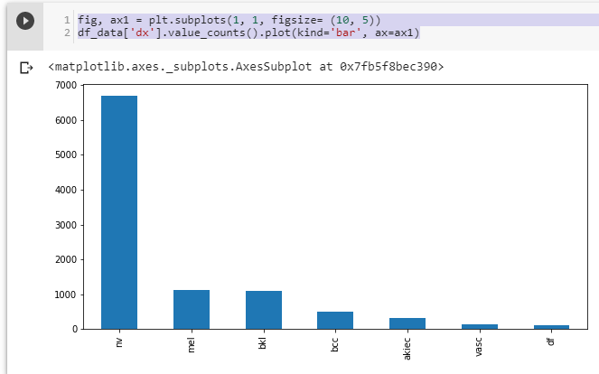
Figure 6. Distribution of all images among classes

In order to classify every class with the same level of accuracy, we need to have an approximately equal number of images for all classes. To ensure this, we use data augmentation techniques. Augmentation is the process of slightly changing images in order to get more training data. For this purpose, we use ImageDataGenerator from the Keras framework, which provides a high- and low-level API for constructing neural networks:

# we are not augmenting the biggest class of 'nv'
class_list = ['mel','bkl','bcc','akiec','vasc','df']
for item in class_list:
    
    aug_dir = 'aug_dir'
    os.mkdir(aug_dir)
    img_dir = os.path.join(aug_dir, 'img_dir')
    os.mkdir(img_dir)
    img_class = item
    img_list = os.listdir('train/' + img_class)
    for fname in img_list:
        shutil.copyfile(
            os.path.join('train/' + img_class, fname), 
            os.path.join(img_dir, fname))
    datagen = ImageDataGenerator(
        rotation_range=180,
        width_shift_range=0.1,
        height_shift_range=0.1,
        zoom_range=0.1,
        horizontal_flip=True,
        vertical_flip=True,
        fill_mode='nearest')
    batch_size = 50
    
    aug_datagen = datagen.flow_from_directory(
        path,
        save_to_dir='train/' + img_class,
        save_format='jpg',
        target_size=(224,224),
        batch_size=batch_size)
    num_aug_images_wanted = 6000 
    
    num_files = len(os.listdir(img_dir))
    num_batches = int(np.ceil((num_aug_images_wanted-num_files)/batch_size))
    for i in range(0,num_batches):
        imgs, labels = next(aug_datagen)
        
    shutil.rmtree('aug_dir')
    
print(str(len(os.listdir('train/nv'))) + ' in nv dir')
print(str(len(os.listdir('train/mel'))) + ' in mel dir')
print(str(len(os.listdir('train/bkl'))) + ' in bkl dir')
print(str(len(os.listdir('train/bcc'))) + ' in bcc dir')
print(str(len(os.listdir('train/akiec'))) + ' in akiec dir')
print(str(len(os.listdir('train/vasc'))) + ' in vasc dir')
print(str(len(os.listdir('train/df'))) + ' in df dir')

The screenshot below shows that images are now more uniformly distributed among all seven classes:

 

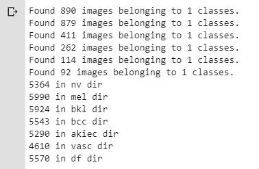
Figure 7. Distribution of images among all seven classes

This particular generator will randomly adjust an image using flip, shift, and zoom techniques according to the parameters we set. In this way, we obtain a sufficient number of images for every class in order to start modeling and training.

Let’s check how our data looks after augmentation on the image below:

# plots images with labels within jupyter notebook
# source: https://github.com/smileservices/keras_utils/blob/master/utils.py
def plots(ims, figsize=(12,6), rows=5, interp=False, titles=None): # 12,6
    if type(ims[0]) is np.ndarray:
        ims = np.array(ims).astype(np.uint8)
        if (ims.shape[-1] != 3):
            ims = ims.transpose((0,2,3,1))
    f = plt.figure(figsize=figsize)
    cols = len(ims)//rows if len(ims) % 2 == 0 else len(ims)//rows + 1
    for i in range(len(ims)):
        sp = f.add_subplot(rows, cols, i+1)
        sp.axis('Off')
        if titles is not None:
            sp.set_title(titles[i], fontsize=16)
        plt.imshow(ims[i], interpolation=None if interp else 'none')
        
plots(imgs, titles=None)

As you can see, we have acquired more images that have only slight differences.

 

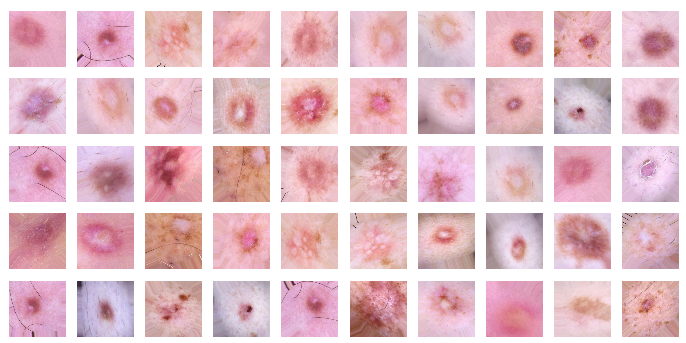
Figure 8. Slightly changed images for training the network

Now the data is ready to be used for deep learning to detect skin cancer, and we can proceed to modeling and training.

Modeling and training the network

As a result of our previous work, we obtained 38,000 images for training. Although we can’t load all of them in memory at once (because of memory limitations), we still want to train the network on all of them. To overcome this issue, let’s use the ImageDataGenerator once again:

train_path = 'train'
valid_path = 'val'
num_train_samples = len(df_train)
num_val_samples = len(df_val)
train_batch_size = 32
val_batch_size = 32
image_size = 224
train_steps = np.ceil(num_train_samples / train_batch_size)
val_steps = np.ceil(num_val_samples / val_batch_size)
datagen = ImageDataGenerator(preprocessing_function= preprocess_input)
train_set = datagen.flow_from_directory(train_path,
                                        target_size=(image_size,image_size),
                                        batch_size=train_batch_size)
val_set = datagen.flow_from_directory(valid_path,
                                      target_size=(image_size,image_size),
                                      batch_size=val_batch_size)
test_set = datagen.flow_from_directory(valid_path,
                                       target_size=(image_size,image_size),
                                       batch_size=1,
                                       shuffle=False)

In this way, the ImageDataGenerator will apply the preprocess_input function to transform images to the format that ResNet152 uses as an input. Then the training data will be generated/loaded from the train_path/valid_path directories.

Sure, the process of loading/unloading images to/from memory brings additional overhead. However, we have no other choice, as our testing environment with 25GB of RAM can’t load all of the images at once.

To solve image classification issues fast and with minimum code, we apply transfer learning techniques. Transfer learning means using a model previously trained for a similar task as a starting point. For our task, we chose the ResNet152 architecture, which was pretrained on the ImageNet dataset. We replaced the top layers with our two fully convolutional layers. ImageNet is a database that consists of millions of images of 1000 classes and is used for developing and testing neural network architectures.

Using Keras, we can load pretrained ImageNet models with only one line of code:

base_model = ResNet152(weights='imagenet', include_top=False)

The parameters above specify that we want to use the ResNet model that’s pretrained on the ImageNet dataset. We set include_top=False to exclude top layers (the classifier) since we won’t use them. Our task is to classify seven types of skin cancer, not the 1000 classes contained in ImageNet. To classify these types of skin cancer, we add two fully convolutional layers (Dense) that work for our dataset:

x = base_model.output
x = GlobalAveragePooling2D()(x)
x = Dense(1000, activation='relu')(x)
x = Dropout(0.25)(x)
predictions = Dense(7, activation='softmax')(x)
model = Model(inputs=base_model.input, outputs=predictions)

The code above is where all experiments happen for modifying the neural network. Improving the results and fighting overfitting (fine-tuning) are usually done with the help of various techniques, layers, and configurations thereof. The topic of fine-tuning is huge and deserves a separate article; therefore, we won’t cover it here.

Since the training process consumes too much time and hardware resources, we have to optimize our time. When solving transfer learning issues, the first question to answer is how many layers we need to train. When it comes to neural networks for image processing, it’s known that the bottom layers of the network learn basic features like colors. The next couple of layers learn lines and curves, the following layers learn shapes, and the last layers learn classes. This is why we don’t always need to retrain the network from scratch.

The more similar your problem is to the problem the pretrained network was originally designed to solve, the fewer layers you’ll have to train. We start with training newly added layers first. To do this, we set all layers of the base_model as non-trainable and recompile the model:

for layer in base_model.layers:
    layer.trainable = False
model.compile(optimizer='rmsprop', loss='categorical_crossentropy', metrics=['accuracy'])

In order to train the network in the most efficient way, we stop training when the network starts to overfit. This indicates that further training will not improve the results for our current configuration. For the purposes of detecting overfit, Keras provides callbacks and even interfaces for implementing callbacks. For our present task, we use standards callbacks:

es_callback1 = EarlyStopping(monitor='val_loss', patience=3)
es_callback2 = EarlyStopping(monitor='val_acc', min_delta=0, patience=10, verbose=1, mode='auto')
filepath="weights-improvement-{epoch:02d}-{val_acc:.2f}.hdf5"
checkpoint = ModelCheckpoint(filepath, monitor='val_acc', verbose=1, save_best_only=True, save_weights_only=False, mode='auto', period=1)

We’ve used three callbacks — es_callback1, es_callback2, and checkpoint — two of which are used to stop training if the model overfits and a third which is the most important one: it freezes the best model so we always have a file with the best weights for our model. Now we can start training:

history = model.fit_generator(train_set, validation_data = val_set, steps_per_epoch = train_steps, initial_epoch = 0, epochs = 10, callbacks = [es_callback1, es_callback2, checkpoint])

When training the top layers, we overfit pretty early — on the 4th epoch — and achieved an accuracy of 81%, which is not bad for a few layers.

WARNING:tensorflow:From /usr/local/lib/python3.6/dist-packages/tensorflow/python/ops/math_grad.py:1250: add_dispatch_support.	<locals>.wrapper (from tensorflow.python.ops.array_ops) is deprecated and will be removed in a future version.
Instructions for updating:
Use tf.where in 2.0, which has the same broadcast rule as np.where
Epoch 1/10
908/908 [==============================] - 256s 282ms/step - loss: 2.3850 - acc: 0.4939 - val_loss: 1.8612 - val_acc: 0.8028
Epoch 00001: val_acc improved from -inf to 0.80277, saving model to weights-improvement-01-0.80.hdf5
Epoch 2/10
908/908 [==============================] - 246s 271ms/step - loss: 1.6444 - acc: 0.5482 - val_loss: 1.7696 - val_acc: 0.8060
Epoch 00002: val_acc improved from 0.80277 to 0.80597, saving model to weights-improvement-02-0.81.hdf5
Epoch 3/10
908/908 [==============================] - 246s 271ms/step - loss: 1.3312 - acc: 0.5988 - val_loss: 1.3410 - val_acc: 0.8102
Epoch 00003: val_acc improved from 0.80597 to 0.81023, saving model to weights-improvement-03-0.81.hdf5
Epoch 4/10
908/908 [==============================] - 246s 271ms/step - loss: 1.1537 - acc: 0.6344 - val_loss: 1.1206 - val_acc: 0.7932
Epoch 00004: val_acc did not improve from 0.81023
Epoch 5/10
908/908 [==============================] - 247s 273ms/step - loss: 1.0781 - acc: 0.6494 - val_loss: 1.5205 - val_acc: 0.6855
Epoch 00005: val_acc did not improve from 0.81023
Epoch 6/10
908/908 [==============================] - 248s 273ms/step - loss: 1.0571 - acc: 0.6584 - val_loss: 1.2620 - val_acc: 0.7921
Epoch 00006: val_acc did not improve from 0.81023
Epoch 7/10
908/908 [==============================] - 248s 274ms/step - loss: 1.0269 - acc: 0.6675 - val_loss: 1.0454 - val_acc: 0.7846
Epoch 00007: val_acc did not improve from 0.81023
Epoch 8/10
908/908 [==============================] - 248s 273ms/step - loss: 1.0345 - acc: 0.6600 - val_loss: 1.2338 - val_acc: 0.7910
Epoch 00008: val_acc did not improve from 0.81023
Epoch 9/10
908/908 [==============================] - 248s 274ms/step - loss: 1.0223 - acc: 0.6610 - val_loss: 1.3205 - val_acc: 0.7495
Epoch 00009: val_acc did not improve from 0.81023
Epoch 10/10
908/908 [==============================] - 249s 274ms/step - loss: 0.9929 - acc: 0.6724 - val_loss: 1.3136 - val_acc: 0.8060
Epoch 00010: val_acc did not improve from 0.81023

Let’s try to train more layers and see what we get. In order to choose how many layers to freeze, we’ve studied the ResNet152 architecture and decided to freeze the whole 5th convolution block:

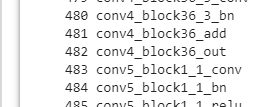
for i, layer in enumerate(base_model.layers):
   print(i, layer.name)

With this command, we can see that ResNet152 has 514 layers and find that the last block starts from 483.

Actually, these are the first steps of fine-tuning the model in order to achieve better results. In this article, we don’t cover all the steps. But we show this one to demonstrate how much influence such steps may have:

for layer in model.layers[:483]:
   layer.trainable = False
for layer in model.layers[483:]:
   layer.trainable = True
from keras.optimizers import Adam
model.compile(optimizer=Adam(lr=0.01), loss='categorical_crossentropy', metrics=['accuracy'])
model.fit_generator(train_set, validation_data = val_set, 
steps_per_epoch = train_steps, epochs = 100, callbacks = [es_callback1, es_callback2, checkpoint])
Epoch 1/100
908/908 [==============================] - 313s 345ms/step - loss: 1.6172 - acc: 0.5986 - val_loss: 0.9165 - val_acc: 0.8326
Epoch 00001: val_acc improved from 0.81023 to 0.83262, saving model to weights-improvement-01-0.83.hdf5
Epoch 2/100
908/908 [==============================] - 304s 334ms/step - loss: 0.9428 - acc: 0.6997 - val_loss: 0.9891 - val_acc: 0.7857
Epoch 00002: val_acc did not improve from 0.83262
Epoch 3/100
908/908 [==============================] - 303s 334ms/step - loss: 0.8702 - acc: 0.7283 - val_loss: 0.9067 - val_acc: 0.8337
Epoch 00003: val_acc improved from 0.83262 to 0.83369, saving model to weights-improvement-03-0.83.hdf5
Epoch 4/100
908/908 [==============================] - 305s 336ms/step - loss: 0.8315 - acc: 0.7458 - val_loss: 1.3260 - val_acc: 0.8102
Epoch 00004: val_acc did not improve from 0.83369
Epoch 5/100
908/908 [==============================] - 305s 336ms/step - loss: 0.7607 - acc: 0.7763 - val_loss: 0.7919 - val_acc: 0.8369
Epoch 00005: val_acc improved from 0.83369 to 0.83689, saving model to weights-improvement-05-0.84.hdf5
Epoch 6/100
908/908 [==============================] - 305s 336ms/step - loss: 0.7269 - acc: 0.7858 - val_loss: 0.8306 - val_acc: 0.8422
Epoch 00006: val_acc improved from 0.83689 to 0.84222, saving model to weights-improvement-06-0.84.hdf5
Epoch 7/100
908/908 [==============================] - 303s 334ms/step - loss: 0.7290 - acc: 0.7800 - val_loss: 1.1973 - val_acc: 0.8188
Epoch 00007: val_acc did not improve from 0.84222
Epoch 8/100
908/908 [==============================] - 303s 334ms/step - loss: 0.6973 - acc: 0.7926 - val_loss: 2.1515 - val_acc: 0.7441
Epoch 00008: val_acc did not improve from 0.84222
	<keras.callbacks.History at 0x7f8ce6f296d8>

On the 6th epoch, we achieved an increase of 3% in accuracy by simply changing the number of layers to train. We can notice that the other callback also worked and saved the best models we obtained so our work is not lost:

Accuracy can be improved even further in so many ways: by adding more data, cleaning up data, changing the model architecture, configuring dropout layers, configuring the regularization of l1 and l2 parameters, changing the learning rate, changing the optimizer, etc. In our next article, we will approach the problem of fine-tuning in order to achieve the best result we can without more data.

Conclusion

Applying deep learning for cancer diagnosis is only one of the numerous ways to use AI for solving medical issues. In this article, we’ve shown an approach to create a network for classifying seven types of skin cancer. Along the way, we overcame a lack of data by slightly changing our images using ImageDataGenerator.

The opportunity to train a network to classify skin cancer is not only exciting but also extremely promising. It shows that medicine can significantly evolve as deep learning technology is improved and optimized for medical purposes.

At Apriorit, we have a team of dedicated developers seasoned in AI, machine learning, and deep learning who are ready to help you improve your project or develop a new one from scratch.

Read more about how AI can enhance your next solution below!