Statistical Methods for Anomaly Detection in Cybersecurity Solutions: Balancing Cost and Efficiency

Key takeaways:

• Statistical anomaly detection costs much less than AI-based detection and adapts better to changes than rule-based methods.
• Statistical methods scale easily and fit into your existing cybersecurity products without big system changes.
• When applied to time-series data, statistical methods can help spot security-critical changes in user behavior.
• Clear, explainable detection logic makes it easier for clients to investigate suspicious activity and respond quickly.

Building an effective anomaly detection system is a balancing act. AI-powered models can deliver strong results but are expensive to implement, while rule-based approaches tend to generate excessive false positives.

However, there’s another approach to anomaly detection that’s often overlooked: statistical analysis methods. They offer a scalable, explainable, and cost-efficient alternative, and they can outperform static rule sets while avoiding the complexity and resource drain of AI. 

If your cybersecurity product needs to detect anomalies in real time without overextending development or operational budgets, a combination of time-series data and statistical analysis may be your answer.

This article explores how statistical methods can be applied to time-series data to build reliable, efficient anomaly detection for cybersecurity solutions — and how Apriorit can help you bring such a system to market.

The role of time-series data in anomaly detection

Before we jump into the actual methodology, let’s first talk about the data that your cybersecurity product needs to spot anomalies in user behavior.

Just flagging a suspicious event isn’t enough for effective anomaly detection. You need context over time. This is where time-series data comes into play, allowing you to capture how user activity evolves and notice deviations from the norm.

Using time-series data as the core of your anomaly behavior engine allows your product to:

• Detect short- and long-term behavioral trends (daily, weekly, seasonal)
• Spot sudden spikes or drops (e.g., bursty access, silent periods)
• Track behavioral drift (e.g., slow escalation in privilege use)
• Power real-time monitoring and alerting mechanisms

For example, time-series data can detect changes in user logins, session times, file downloads, and other events that can indicate malicious activity. It’s only possible for your cybersecurity platform to notice these deviations when you analyze user behavior in sequence and across time. 

But how can you enable your system to detect anomalies automatically? There are several ways to implement this, including through statistical analysis, AI-powered detection, a cluster-based approach, or a rule-based system. 

In the next section, we discuss these key anomaly detection methods and explain why a statistical approach, while less common, can offer you superior cost-efficiency, explainability, and scalability.

4 ways to detect anomalies in time-series data

There are four main approaches to anomaly detection in time-series data:

• Rule-based
• Cluster-based
• AI/ML-based
• Statistical

Each of these approaches has its trade-offs in terms of cost, complexity, accuracy, and explainability.

Table 1. Approaches to implementing anomaly behavior detection 

Among these four, statistical methods are the least common for detecting anomalies. However, our practice shows that these methods have great potential for striking a balance between explainability, speed, and a low level of false positives. Let’s discuss why statistical methods might be suitable for your cybersecurity product.

Read also

Implementing Artificial Intelligence and Machine Learning in Cybersecurity Solutions

Leverage the power of AI and ML for your cybersecurity solution. Discover the benefits, limitations, and use cases of these cutting-edge technologies.

Learn more

Why use statistical methods for anomaly detection?

Statistical methods are designed to flag extreme values in data. They are efficient, simple to implement, and provide interpretable results. 

Working with statistical methods, your team can identify behavioral anomalies like login spikes, off-hours access patterns, and other potential indicators of malicious activity.

To assess whether detecting anomalies with statistical methods is a suitable solution for your case, you need to account for factors like the quality and volume of available data, the variety of threats your product may face, required analysis speed, and so on.

You should consider using statistical methods if:

• You need a scalable and explainable system that can easily integrate with your existing product
• Your resources and data are insufficient for training an AI model
• Your top priorities are real-time monitoring and clear insights
• You want a cost-effective solution that avoids investing in costly infrastructure
• You prioritize a fast time to market and delivering results quickly
• You need a foundation for your anomaly detection system that can later be paired with AI or clustering methods

You should consider other methods if:

• Your cybersecurity product deals with advanced, stealthy threats that target high-value data or systems. In this case, AI-based anomaly detection may be a better fit.
• Behavior patterns shift rapidly, and your system has to constantly adapt to them. AI systems are best at quickly adapting and dealing with complex patterns.
• Your threats are well-defined and compliance-driven. In this case, you’ll be better suited with rule-based methods that can quickly enforce strict rules.
• You’re dealing with large, unlabeled datasets in a complex environment. In this case, opt for cluster-based methods that can group users or behaviors into natural patterns without any predefined baselines.

If you feel like statistical methods best suit your needs, consider combining several variations to achieve higher precision and speed in anomaly detection. In the next section, we cover the methods that Apriorit commonly uses within cybersecurity projects and discuss specific applications for each.

4 statistical methods for anomaly detection, with practical examples

There are several widely used statistical methods for detecting anomalies. The most common include:

• Z-score
• Interquartile Range (IQR)
• Median Absolute Deviation (MAD)
• Kernel Density Estimation (KDE)

In this section, we talk about these methods in detail and test them using a synthetic dataset with a known offset. 

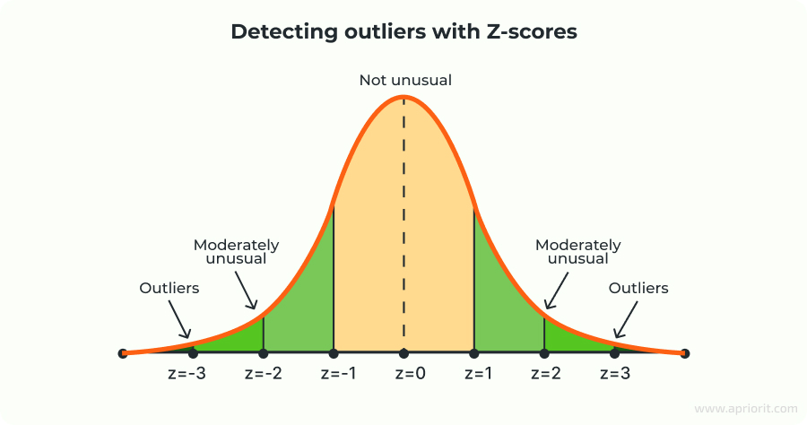
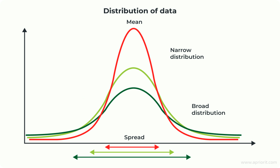
Z-score 

A Z-score is a special number that tells us how far away a data point is from the usual or average. It tells the equivalent of whether you did something really well, just okay, or not so great compared to everyone else. 

Using the Z-score method, we identify any instances where the absolute value of the Z-score is over a given threshold. This is the formula for calculating the Z-score: 

Here’s what each component means: 

• Z is the Z-score we’re calculating. 
• X is the data point we want to evaluate. 
• μ (mu) is the mean (average) of the dataset. 
• σ (sigma) is the standard deviation, which measures how spread out the data is. 

This method works well for normally distributed data and is straightforward to implement and interpret.

Example: 

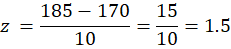
Say you have data on the number of calls made by a group of users per day. The average (mean) number is 170, and the standard deviation is 10. You want to calculate the Z-score for someone who made 185 calls.

Using the Z-score formula:

Where:

• X = 185 (individual’s number of calls)
• μ = 170 (mean)
• σ = 10 (standard deviation)

Result: A user who made 185 calls has a Z-score of 1.5, meaning their number of calls is 1.5 standard deviations above the mean. This indicates that the value is somewhat unusual, but not extremely rare.

Code example:

def calculate_z_scores_manual(data): 
	""" 
	Calculates Z-scores manually for a given dataset. 
	Args: 
    	data (list or numpy.ndarray): The input dataset. 
	Returns: 
    	list: A list of Z-scores for each data point. 
	""" 
	mean = np.mean(data) 
	std_dev = np.std(data) 
 
	if std_dev == 0:  # Handle the case of zero standard deviation 
    	return [0.0] * len(data) 
 
	z_scores = [(x - mean) / std_dev for x in data] 
	return z_scores

def calculate_z_scores_manual(data): 
	""" 
	Calculates Z-scores manually for a given dataset. 
	Args: 
    	data (list or numpy.ndarray): The input dataset. 
	Returns: 
    	list: A list of Z-scores for each data point. 
	""" 
	mean = np.mean(data) 
	std_dev = np.std(data) 
 
	if std_dev == 0:  # Handle the case of zero standard deviation 
    	return [0.0] * len(data) 
 
	z_scores = [(x - mean) / std_dev for x in data] 
	return z_scores

Read also

How to Detect Vulnerabilities in Software When No Source Code Is Available

Find out how dynamic fuzzing can help your team detect vulnerabilities that traditional testing methods miss.

Learn more

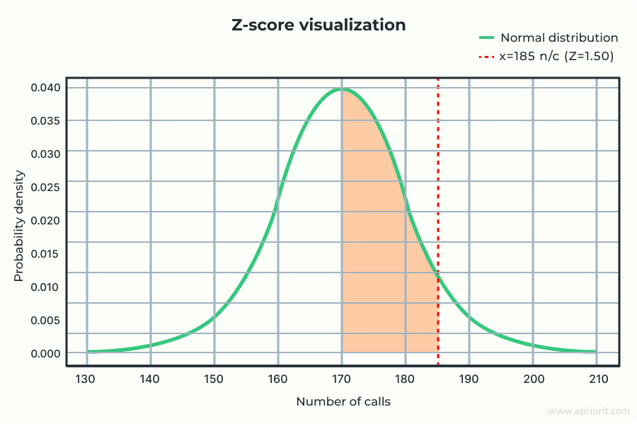
Interquartile range (IQR) 

A widely used and statistically robust method for identifying extreme values is the interquartile range (IQR). One of the main advantages of IQR over Z-scores is its resistance to outliers. 

While Z-scores rely on the mean and standard deviation, which can be skewed by extreme values, IQR uses the median and quartiles. This makes IQR more reliable when dealing with skewed or non-normal distributions.

To calculate IQR, follow these steps:

1. Find the first quartile (Q1) — the 25th percentile
2. Find the third quartile (Q3) — the 75th percentile
3. Compute IQR using this formula:

Using IQR, you can define thresholds to identify outliers:

• Lower bound

• Upper bound

Here, 1.5 is the IQR coefficient we chose. 

The value of the coefficient determines the sensitivity of outlier detection. Using a small coefficient like 1.5 results in tight boundaries, which cause more data points to be identified as outliers, including some normal variations. This approach can lead to more false positives but is helpful when it’s important to detect even minor deviations. 

On the other hand, a larger coefficient such as 2.2 creates wider boundaries, decreasing sensitivity to small fluctuations and reducing the number of false positives. However, this might cause some subtle anomalies to go unnoticed (i.e. false negatives). 

Ultimately, the right coefficient depends on your data characteristics and whether you want to prioritize catching anomalies or avoiding false positives. 

Example: 

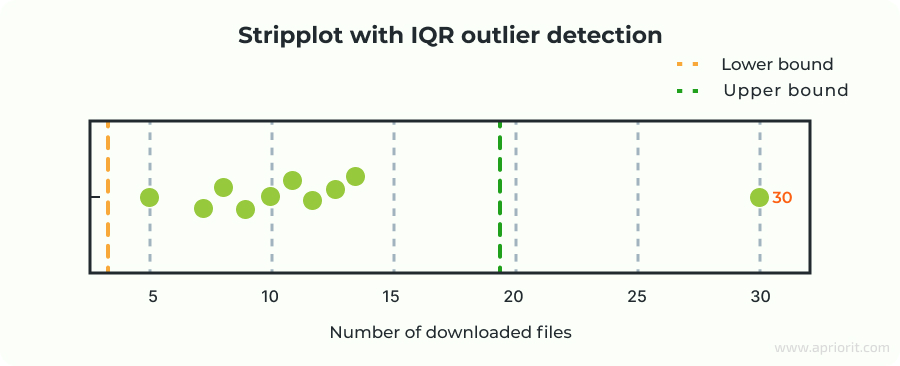
Imagine you have data on the number of files downloaded by users in a month:

[5, 7, 8, 9, 10, 11, 12, 13, 14, 30]

Let’s check if 30 is an outlier using the IQR method.

1. Sort the data (already sorted above).
2. Calculate Q1 and Q3:
   
   • Q1 = 8
   • Q3 = 13
     
3. Compute the IQR:

Q3 − Q1 = 13 − 8 = 5.

4. Calculate the bounds using k = 1.5:
   
   • Lower bound = Q1 − 1.5 × IQR = 8 − 7.5 = 0.5
   • Upper bound = Q3 + 1.5 × IQR = 13 + 7.5 = 20.5.
     

In this case, any data point below 0.5 or above 20.5 is considered an outlier.

Result: Since 30 > 20.5, it is flagged as an outlier by the IQR method.

Code example:

import numpy as np 
 
def calculate_iqr_scores(data): 
	""" 
	Calculates IQR-based scores for outlier detection. 
	Args: 
    	data (list or numpy.ndarray): The input dataset. 
	Returns: 
    	list: A list of IQR scores (how far each point is from Q1-Q3 range). 
	""" 
	q1 = np.percentile(data, 25) 
	q3 = np.percentile(data, 75) 
	iqr = q3 - q1 
 
	lower_bound = q1 - 1.5 * iqr 
	upper_bound = q3 + 1.5 * iqr 
 
	# Score: 0 if in range, else absolute distance from nearest bound 
	scores = [] 
	for x in data: 
    	if x < lower_bound: 
        	scores.append(lower_bound - x) 
    	elif x > upper_bound: 
        	scores.append(x - upper_bound) 
    	else: 
        	scores.append(0.0) 
	return scores

import numpy as np 
 
def calculate_iqr_scores(data): 
	""" 
	Calculates IQR-based scores for outlier detection. 
	Args: 
    	data (list or numpy.ndarray): The input dataset. 
	Returns: 
    	list: A list of IQR scores (how far each point is from Q1-Q3 range). 
	""" 
	q1 = np.percentile(data, 25) 
	q3 = np.percentile(data, 75) 
	iqr = q3 - q1 
 
	lower_bound = q1 - 1.5 * iqr 
	upper_bound = q3 + 1.5 * iqr 
 
	# Score: 0 if in range, else absolute distance from nearest bound 
	scores = [] 
	for x in data: 
    	if x < lower_bound: 
        	scores.append(lower_bound - x) 
    	elif x > upper_bound: 
        	scores.append(x - upper_bound) 
    	else: 
        	scores.append(0.0) 
	return scores

Median absolute deviation (MAD) 

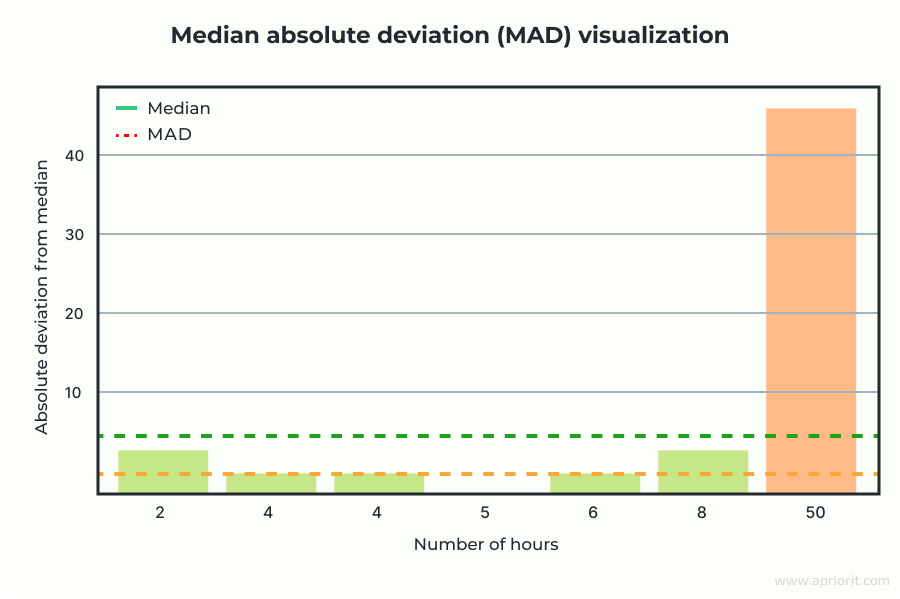
The median absolute deviation is another robust measure of spread. It is often preferred when working with skewed data or datasets containing outliers. Like IQR, MAD focuses on the median rather than the mean, making it resistant to the influence of extreme values.

To detect outliers using MAD, you need to:

1. Calculate the median of the dataset.
2. Compute the absolute deviation of each data point from the median.
3. Find the median of those absolute deviations — this is the MAD.
4. To assess whether a data point is an outlier, calculate its MAD score:

Where:

• X_i is each individual value in the dataset
• Median (X) is the median value of the entire dataset X_i
• |X_i – median (X)| is the absolute deviation of a given value from the median of the dataset. It measures how far the value is from the median, regardless of the direction (positive or negative).

After you calculate the MAD score for a data point, you need to compare it to a threshold — often 3.5 or higher. If the score exceeds the threshold, the data point is flagged as an outlier.

The statistical methods discussed above are designed to detect extreme values, but they can miss a different type of outlier called an internal outlier. These outliers aren’t far from the rest of the data in terms of range but still stand out due to the overall distribution. They typically appear in datasets with gaps or multiple peaks.

Example: 

Suppose you have the following dataset representing the number of hours a group of people has been using a particular feature: 

X = [2, 4, 4, 5, 6, 8, 50]

1. Calculate the median of X:

median(X) = 5

2. Calculate the absolute deviations from the median:

|X_i – median (X)| = [|2 – 5], |4 – 5|, |5 – 5|, |8 – 5|, |50 – 5|] = [3, 1, 1, 0, 1, 3, 45]

3. Calculate the MAD:

MAD = median([3,1,1,0,1,3,45]) = 1

Although 50 is not far from the IQR boundary in this example, it clearly stands apart from the rest of the values. Since this score is much higher than the common threshold (3.5), 50 is identified as an outlier.

Code example: 

import numpy as np 
 
def calculate_mad_scores(data): 
	""" 
	Calculates MAD-based scores for each data point. 
	Args: 
    	data (list or numpy.ndarray): The input dataset. 
	Returns: 
    	list: A list of MAD scores for each point. 
	""" 
	median = np.median(data) 
	abs_deviation = np.abs(data - median) 
	mad = np.median(abs_deviation) 
 
	if mad == 0: 
    	return [0.0] * len(data) 
 
	mad_scores = [(x - median) / mad for x in data] 
	return mad_scores

import numpy as np 
 
def calculate_mad_scores(data): 
	""" 
	Calculates MAD-based scores for each data point. 
	Args: 
    	data (list or numpy.ndarray): The input dataset. 
	Returns: 
    	list: A list of MAD scores for each point. 
	""" 
	median = np.median(data) 
	abs_deviation = np.abs(data - median) 
	mad = np.median(abs_deviation) 
 
	if mad == 0: 
    	return [0.0] * len(data) 
 
	mad_scores = [(x - median) / mad for x in data] 
	return mad_scores

Read also

How and Why Should You Build a Custom XDR Security Platform?

Discover how custom XDR solutions can protect your business from sophisticated attacks. Explore our valuable insights into the benefits of XDR and build a tailored solution to meet your unique security needs.

Learn more

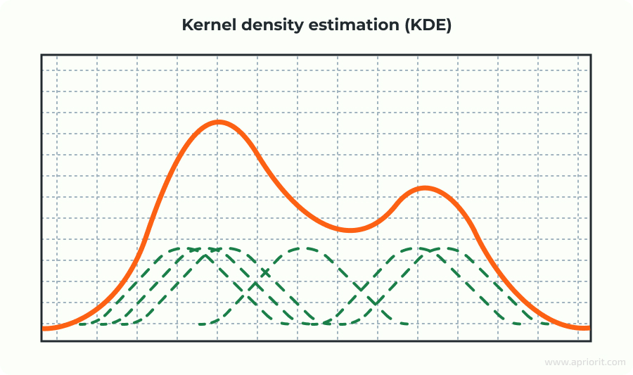
Kernel Density Estimation (KDE) 

Kernel density estimation is more flexible with unusual or irregular distributions than the previous methods. It estimates the underlying probability density function of your data rather than assuming a specific distribution.

To calculate KDE, the algorithm places a small kernel — a shape like a triangle, box, or Gaussian curve — on each data point. Where data points are close together, their kernels overlap strongly, producing a high density estimate. In sparse regions, fewer kernels overlap, so the estimate is lower. 

This results in a smooth curve showing the relative likelihood of where data points are expected to occur. If no data points are near a given value, the estimated probability density at that value is zero, meaning such values are very unlikely.

After calculating the KDE, we apply the IQR method to detect outliers.

To calculate an anomaly score with any method, we first need to create features that capture key aspects of user activity and interaction patterns, such as number of daily logins, frequency of actions, activity times, or properties of accessed resources like domain name lengths. 

These features help anomaly detection models learn what normal behavior looks like and identify deviations. Well-crafted features significantly improve the accuracy and interpretability of anomaly detection.

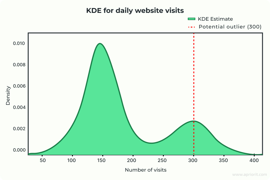
Example: 

Suppose you have daily website visit counts for a small online store:

 [120, 135, 140, 150, 155, 160, 162, 170, 175, 300].

To check if 300 is an outlier, you estimate the distribution using KDE. Most values fall between 120 and 175, forming a high-density region. The value 300 lies far outside this region, where the KDE density is low — indicating it’s rare or anomalous. 

By visualizing the KDE curve, you can clearly see that 300 corresponds to a very low probability, confirming it as an outlier.

Code example: 

from scipy.stats import gaussian_kde 
 
 
def calculate_kde_scores(data): 
	""" 
	Calculates density-based scores using KDE. Lower values indicate more "anomalous". 
	Args: 
    	data (list or numpy.ndarray): The input dataset. 
	Returns: 
    	list: Inverse KDE scores (lower density = higher anomaly). 
	""" 
	kde = gaussian_kde(data) 
	densities = kde.evaluate(data) 
 
	# Optionally: return inverse of density as anomaly score 
	kde_scores = [1.0 / d if d > 0 else float('inf') for d in densities] 
	return kde_scores 

from scipy.stats import gaussian_kde 
 
 
def calculate_kde_scores(data): 
	""" 
	Calculates density-based scores using KDE. Lower values indicate more "anomalous". 
	Args: 
    	data (list or numpy.ndarray): The input dataset. 
	Returns: 
    	list: Inverse KDE scores (lower density = higher anomaly). 
	""" 
	kde = gaussian_kde(data) 
	densities = kde.evaluate(data) 
 
	# Optionally: return inverse of density as anomaly score 
	kde_scores = [1.0 / d if d > 0 else float('inf') for d in densities] 
	return kde_scores 

Now that we have discussed the main statistical methods for anomaly detection, let’s look at how you can use them for your own anomaly detection system.

Read also

Anomaly Detection on Social Media: How to Build an AI-Powered SaaS Platform with Python Tools

Develop a smart anomaly detection solution. Learn who can benefit from such a solution and how to use AI and Python to create a SaaS media monitoring platform for your customers.

Learn more

How to use statistical methods for anomaly detection: a step-by-step guide

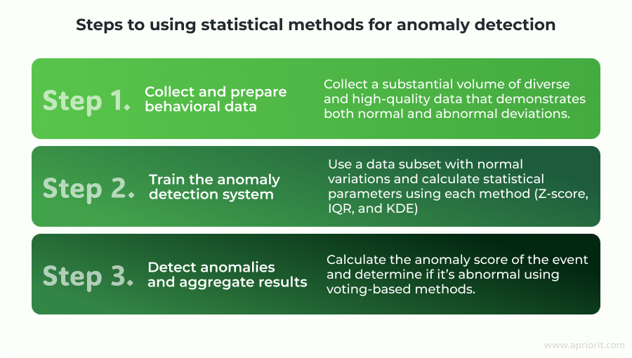
Step 1. Collect and prepare behavioral data

Before applying statistical methods, your anomaly detection system needs a solid baseline of what “normal” looks like. The first step is collecting and preparing high-quality data. This will ensure the system can accurately model typical behavior and reliably detect deviations.

Let’s discuss what properties your data should have to serve as a foundation for your anomaly detection system. 

1. Data quality

Accurate, complete, and consistent data is critical. Low-quality data can lead to false positives or false negatives (i.e. missed anomalies). Therefore, it’s essential to verify data sources, validate data integrity, and clean up any errors, outliers, or missing values before applying anomaly detection techniques in cybersecurity solutions.

2. Data quantity

The quantity of data is a factor of both the volume of data and the frequency with which it is collected. The quantity of data you’ll need to collect depends on the complexity of your system. Dynamic systems typically require larger datasets to accurately model normal behavior and minimize uncertainty.

Conversely, for stable and predictable systems, a smaller amount of data may be sufficient to detect unusual patterns. 

3. Data diversity

The data you collect should be diverse enough to reflect the full range and variety of system behavior. 

For instance, when analyzing potential fraud in online transactions, incorporating data from various sources — such as user behavior, payment details, IP addresses, and browsing history — can offer a more comprehensive understanding. Data diversity also increases the likelihood of uncovering previously unseen or subtle anomalies that might be missed if only a single data source is used. 

Best practices for building statistical features

Features are the individual measurable properties or characteristics of the data you’re analyzing. In statistical anomaly detection, features are typically numerical values that represent behavior as users interact with digital systems such as websites, applications, or online platforms.

User behavior may include actions like clicking buttons, viewing pages, logging in, submitting forms, performing transactions, or navigating through interface elements. Features may include time of day (e.g., time in 24-hour format), session duration (in seconds), or number of clicks.

In general, statistical methods work best with features that show variation and continuity, as this allows for effective modeling of data distributions. Here are best practices you can use to ensure your feature formats work with specific statistical methods.

1. Use continuous or granular features instead of Boolean values

Statistical methods like Z-score or KDE depend on data variability to effectively model distributions. Boolean features (e.g., 0/1 or true/false) offer limited variation and may reduce detection accuracy. Whenever possible, replace binary indicators with more informative alternatives. For example, use weekday (0–6) instead of a simple is_weekend flag.

2. Сhoose features with natural variation

Your features should capture a range of values. For example:

• domain_length (length of the domain name)
• session_duration (in seconds)
• number_of_clicks

These features offer more insight than simple flags or binary variables.

3. Encode categorical variables wisely

If you need to encode categorical variables, prefer techniques like ordinal encoding (if the order matters) or frequency encoding instead of one-hot encoding to preserve numerical variation.   

In conclusion, the more detailed and variable your features are, the more effective your statistical methods will be at identifying outliers.

Related project

Improving a SaaS Cybersecurity Platform with Competitive Features and Quality Maintenance

Learn how you can elevate a SaaS-based cybersecurity platform to meet the highest industry standards with our assistance. We helped our client implement new features, fix bugs, and improve their platform’s UI/UX, resulting in increased stability and competitiveness.

Project details

Step 2. Train the anomaly detection system

Although we aren’t using AI, we still need to train our system. To do this, we use a subset of data to compute the necessary parameters for each anomaly detection method. These parameters are saved to separate files corresponding to event types and are later used for real-time anomaly detection. 

To train statistical methods such as Z-score, IQR, or KDE for anomaly detection, follow these steps: 

1. Select a training subset

Use a subset of the data that mostly contains normal (non-anomalous) events. This subset serves as a training dataset and provides a baseline for learning typical behavior patterns. To achieve this, the dataset retrieved from the database is divided into two parts: one for training and another for anomaly detection (or evaluation). 

Before applying any detection methods, it’s important to preprocess the data and compute all necessary features, such as time-based statistics, frequency counts, or domain-specific metrics. The quality and completeness of these features will directly impact the accuracy of the anomaly detection model. 

Additionally, it’s essential to ensure that the training data is not contaminated with anomalies, as they may distort the model’s understanding of “normal” behavior. Ideally, the training period should represent typical system behavior under stable conditions. 

2. Calculate parameters 

For each feature, calculate the statistical parameters needed for the method:

• For Z-score, compute mean (mean) and standard deviation (std). 
• For IQR, compute the lower bound (lower) and upper bound (upper). 
• For KDE, compute the log of event density (log_density). Then apply the IQR method to these density values, using the lower and upper bounds (based on percentiles), to detect anomalies.

3. Save the parameters 

Store the computed parameters in dedicated files or databases (e.g., in CSV format) so they can be reused later without retraining. Let’s demonstrate saving parameters for logon events using the Z-score method:

{  
	"user": "patrick",  
	"weekday: 0,  
	"date": "2024-06-18 11:52:14"  
  }

{  
	"user": "patrick",  
	"weekday: 0,  
	"date": "2024-06-18 11:52:14"  
  }

In this data, we can see the user name, the weekday (0 indicates Monday), and the date when the login event occurred. This means that the feature name is weekday and its value is 0. For these entries, we calculate the mean and standard deviation, and we save these parameters (along with the feature label) for future use in calculating anomaly scores. 

{  
	"user": "patrick",  
	"mean": 1.666667,  
	"std": 1.4906,  
	"feature_name": "weekday",  
	"date_training": "2024-06-18 12:52:14"  
  }

{  
	"user": "patrick",  
	"mean": 1.666667,  
	"std": 1.4906,  
	"feature_name": "weekday",  
	"date_training": "2024-06-18 12:52:14"  
  }

Table 2. Definitions of stored feature parameters 

This data is saved for later use in anomaly detection. We store the calculated parameters from the training data (such as mean, standard deviation, IQR, or KDE distributions) and use them as reference points for scoring anomalies. Each anomaly detection method relies on these saved parameters to compute an anomaly score for new incoming data. 

By reusing the parameters derived from normal behavior, we ensure consistent and efficient evaluation during the detection phase. This approach also allows the system to scale, as it avoids recalculating baselines for each new dataset and allows the system to detect deviations in real-time or batch analysis.

Read also

How to Enhance Your Cybersecurity Platform: XDR vs EDR vs SIEM vs IRM vs SOAR vs DLP

Learn about the benefits and limitations of different types of cybersecurity platforms and discover how you can integrate them into your product to cover your users’ cybersecurity needs.

Learn more

Step 3. Detect anomalies and aggregate results 

After receiving an event, we calculate the anomaly score using each method for each feature and save the results to dedicated files or databases (e.g., in CSV format). Once all anomaly scores are calculated, we apply voting methods to combine the results from all statistical methods. 

Here is an example of anomaly score results for a domain length feature:

{ 
"session_id": 1, 
"user_id": 1, 
"user": "patrick", 
"date": "2024-05-12 12:21:56.557000000", 
"date_only": "2024-05-12", 
"domain_length": 34.0, 
"z_score": 1.0, 
"iqr": 1, 
"kde": 1 
}

{ 
"session_id": 1, 
"user_id": 1, 
"user": "patrick", 
"date": "2024-05-12 12:21:56.557000000", 
"date_only": "2024-05-12", 
"domain_length": 34.0, 
"z_score": 1.0, 
"iqr": 1, 
"kde": 1 
}

In this case, we can see that in the HTTP event, the user tried to access a long domain that is not typical for them, and all three methods detected this event as an anomaly. 

Here are the voting-based methods: 

• Majority voting — flags as anomaly if most methods agree 
• Weighted voting — assigns weights based on method reliability/performance 
• Unanimous voting — requires all methods to agree (high precision, low recall) 

Majority voting is an ensemble method in machine learning where multiple models (classifiers) independently make predictions, and the final class is selected as the one that receives the most votes from all models. 

def majority_vote(self, df: pd.DataFrame) -> pd.DataFrame: 
	""" 
	Determines the majority vote across specified columns in a DataFrame. 
	Returns the most frequent value in each row. 
	""" 
	df['majority'] = df[self.columns].mode(axis=1)[0] 
	return df

def majority_vote(self, df: pd.DataFrame) -> pd.DataFrame: 
	""" 
	Determines the majority vote across specified columns in a DataFrame. 
	Returns the most frequent value in each row. 
	""" 
	df['majority'] = df[self.columns].mode(axis=1)[0] 
	return df

Weighted voting is a variation of the majority voting ensemble method in machine learning, where each model (classifier) contributes to the final decision with a certain weight based on its performance or reliability. Instead of each model having equal influence, models that perform better (e.g., have higher accuracy or a lower error rate) are given more weight in the voting process. 

Weight_map = {‘z_score’: 1, ‘iqr’: 2, ‘kde’: 3} 
def weighted_vote(row, weights): 
	score = {} 
	for col, weight in weights.items(): 
        val = row[col] 
    	score[val] = score.get(val, 0) + weight 
	return max(score.items(), key=lambda x: x[1])[0] 
 
def weighted_result(self, df: pd.DataFrame) -> pd.DataFrame: 
	""" 
	Computes a weighted vote per row using a predefined weight map. 
	Applies custom weights to the values in each row based on vote type. 
	""" 
	df['weighted_vote'] = df.apply(lambda row: Results.weighted_vote(row, weight_map), axis=1) 
	return df

Weight_map = {‘z_score’: 1, ‘iqr’: 2, ‘kde’: 3} 
def weighted_vote(row, weights): 
	score = {} 
	for col, weight in weights.items(): 
        val = row[col] 
    	score[val] = score.get(val, 0) + weight 
	return max(score.items(), key=lambda x: x[1])[0] 
 
def weighted_result(self, df: pd.DataFrame) -> pd.DataFrame: 
	""" 
	Computes a weighted vote per row using a predefined weight map. 
	Applies custom weights to the values in each row based on vote type. 
	""" 
	df['weighted_vote'] = df.apply(lambda row: Results.weighted_vote(row, weight_map), axis=1) 
	return df

Unanimous voting is a strict ensemble method in which a class label is assigned only if all models (classifiers) in the ensemble make the same prediction. If there is any disagreement among models, no prediction is made (or an alternative strategy is used, such as abstaining or defaulting to a fallback decision).

def unanimous_vote(self, df: pd.DataFrame) -> pd.DataFrame: 
	""" 
	Determines the unanimous vote across specified columns in a DataFrame. 
	Returns the value if all values in the row are the same, otherwise marks as non-unanimous. 
	""" 
	df['unanimous'] = df[self.columns].apply(lambda row: row.iloc[0] if row.nunique() == 1 else None, axis=1) 
	return df

def unanimous_vote(self, df: pd.DataFrame) -> pd.DataFrame: 
	""" 
	Determines the unanimous vote across specified columns in a DataFrame. 
	Returns the value if all values in the row are the same, otherwise marks as non-unanimous. 
	""" 
	df['unanimous'] = df[self.columns].apply(lambda row: row.iloc[0] if row.nunique() == 1 else None, axis=1) 
	return df

Then we combine the results from all features. If any feature is marked as anomalous on a given date, we mark the entire event as an anomaly. For summarizing results, we generally use a weighted vote by assigning weights to all methods. 

This is an example of results for the HTTP event: 

{  
"user": "patrick",  
"date": "2024-05-12 10:05:17.539999200", 
"hour_bucket": 1.0,  
	"user_id": 1,  
	"working_hours": 0,  
   "session_id": 1,  
	"weekday": 0.0,  
	"http_new_domain_count": 1,  
	"anomaly_score": 1.0  
}

{  
"user": "patrick",  
"date": "2024-05-12 10:05:17.539999200", 
"hour_bucket": 1.0,  
	"user_id": 1,  
	"working_hours": 0,  
   "session_id": 1,  
	"weekday": 0.0,  
	"http_new_domain_count": 1,  
	"anomaly_score": 1.0  
}

As you can see, after we calculated the results using a weighted vote, four features (hour_bucket, user_id, session_id, and http_new_domain_count) were flagged as anomalies (assigned a value of 1). Since there were multiple flagged features, the system flagged the whole HTTP event as an anomaly. 

This approach of combining multiple statistical analysis methods allows us to avoid false positives with more certainty and build a reliable anomaly detection mechanism.

Conclusion

Anomaly detection in time-series data based on statistical methods offers a reliable and efficient way to monitor system behavior, identify unusual activity, and enhance the security posture of digital solutions. 

Each statistical method we covered above offers a different way to identify outliers. Z-scores work well with normally distributed data, while IQR and MAD are more robust at handling extreme values and better suited for skewed data. KDE provides flexibility for complex or multimodal distributions and helps detect internal outliers. 

By choosing the method that aligns with your data’s characteristics and combining it with well-designed features, you can more effectively detect anomalies and gain meaningful insights.

At Apriorit, we help cybersecurity vendors and SaaS providers design and implement robust anomaly detection systems tailored to their product architecture and use cases. 

We can help you:

• Choose the most relevant technologies and methods for anomaly detection depending on your project’s specifics
• Design and engineer a cybersecurity product from the ground up using our secure SDLC methods that keep security at the forefront of all development stages 
• Integrate reliable security features into your existing cybersecurity platform
• Implement AI features where they are feasible and relevant to your needs, or suggest and integrate suitable non-AI alternatives

Our outstanding portfolio of cybersecurity projects demonstrates our ability to deliver secure, scalable, and high-performing solutions. 

Whether you’re building a new cybersecurity product or upgrading an existing one, our team is ready to support your innovation.