Skip to main content

People recognize and distinguish each other’s voices almost immediately. But what comes naturally for a human is challenging for a machine learning (ML) system. To make your speaker recognition solution efficient and performant, you need to carefully choose a model and train it on the most fitting dataset with the right parameters.
In this article, we briefly overview the key speaker recognition approaches along with tools, techniques, and models you can use for building a speaker recognition system. We also analyze and compare the performance of these models when configured with different parameters and trained with different datasets. This overview will be useful for teams working on speech processing and AI-powered speech emotion recognition.
Contents:
Understanding the basics of speaker recognition
Like a person’s retina and fingerprints, a person’s voice is a unique identifier. That’s why speaker recognition is widely applied for building human-to-machine interaction and biometric solutions like voice assistants, voice-controlled services, and speech-based authentication products.
To provide personalized services and correctly authenticate users, such systems should be able to recognize a user. To do so, modern speech processing solutions often rely on speaker recognition.
Speaker recognition verifies a person’s identity (or identifies a person) by analyzing voice characteristics.
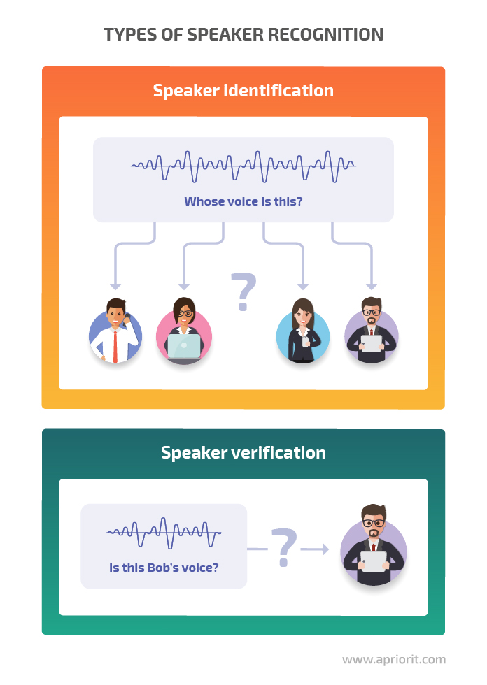
There are two types of speaker recognition:
- Speaker identification — The system identifies a speaker by comparing their speech to models of known speakers.
- Speaker verification — The system verifies that the speaker is who they claim to be.
You can build a speaker recognition system using static signal processing, machine learning algorithms, neural networks, and other technologies. In this article, we focus on the specifics of accomplishing speaker recognition tasks using machine learning algorithms.
Both speaker verification and speaker identification systems consist of three main stages:
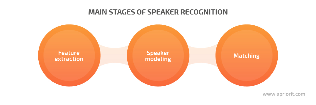
- Feature extraction is when the system extracts essential voice features from raw audio
- Speaker modeling is when the system creates a probabilistic model for each speaker
- Matching is when the system compares the input voice with every previously created model and chooses the model that best matches the input voice
Implementing each of these stages requires different tools and techniques. We look closely at some of them in the next section.
Looking to develop speaking recognition functionality?
Delegate all your complex tasks to Apriorit’s experts in artificial intelligence and machine learning to receive the exact features your software needs!
Speech recognition techniques and tools
Speech is the key element in speaker recognition. And to work with speech, you’ll need to reduce noise, distinguish parts of speech from silence, and extract particular speech features. But first, you’ll need to properly prepare your speech recordings for further processing.
Speech signal preprocessing
Converting speech audio to the data format used by the ML system is the initial step of the speaker recognition process.
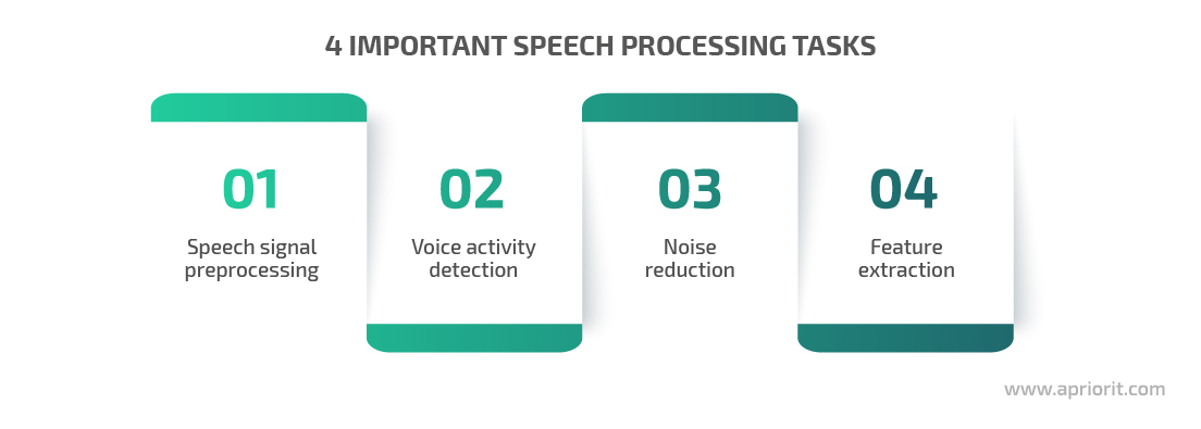
Start by recording speech with a microphone and turning the audio signal into digital data with an analog-to-digital converter. Further signal processing commonly includes processes like voice activity detection (VAD), noise reduction, and feature extraction. We’ll look at each of these processes later.
First, let’s overview some of the key speech signal preprocessing techniques: feature scaling and stereo-to-mono conversion.
Since the range of signal values varies widely, some machine learning algorithms can’t properly recognize audio without normalization. Feature scaling is a method used to normalize the range of independent variables or features of data. Scaling data eliminates sparsity by bringing all your values onto the same scale, following the same concept as normalization and standardization.
For example, you can standardize your audio data using the sklearn.preprocessing package. It contains utility functions and transformer classes that allow you to improve the representation of raw feature vectors.
Here’s how this works in practice:
from sklearn import preprocessing
def extract_features(audio,rate):
   mfcc_feature = mfcc.mfcc(audio,rate, winlen=0.020,preemph=0.95,numcep=20,nfft=1024,ceplifter=15,highfreq=6000,nfilt=55,appendEnergy=False)
   mfcc_feature = preprocessing.scale(mfcc_feature)
   delta = calculate_delta(mfcc_feature)
   combined = np.hstack((mfcc_feature,delta))
return combinedThe number of channels in an audio file can also influence the performance of your speaker recognition system. Audio files can be recorded in mono or stereo format: mono audio has only one channel, while stereo audio has two or more channels. Converting stereo recordings to mono helps to improve the accuracy and performance of a speaker recognition system.
Python provides a pydub module that enables you to play, split, merge, and edit WAV audio files. This is how you can use it to convert a stereo WAV file to a mono file:
from pydub import AudioSegment
mysound = AudioSegment.from_wav("stereo_infile.wav")
# set mono channel
mysound = mysound.set_channels(1)
# save the result
mysound.export("mono_outfile.wav", format="wav")Now that we’ve overviewed key preparation measures, we can dive deeper into the specifics of speech signal processing techniques.
Voice activity detection
To let the feature extraction algorithm for speaker recognition focus only on speech, we can remove silence and non-speech parts of the audio. This is where VAD comes in handy. This technique can distinguish human speech from other signals and is often used in speech-controlled applications and devices like voice assistants and smartphones.
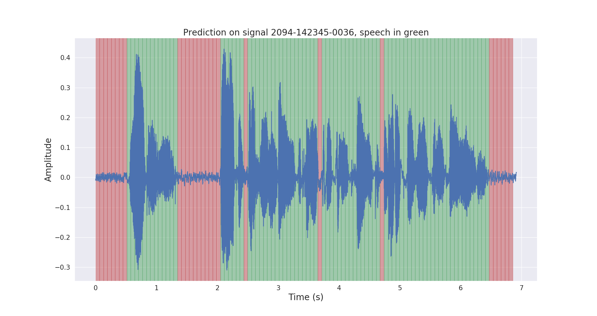
The main goal of a voice activity detection algorithm is to determine which segments of a signal are speech and which are not. A VAD algorithm can improve the performance of a speaker verification system by making sure that the speaker’s identity is calculated using only the frames that contain speech. Therefore, you should evaluate the necessity of using a VAD algorithm to overcome problems in designing a robust speaker verification system.
As for the practical aspects of VAD implementation, you can turn your attention to PyTorch, a high-performance open-source library with a rich variety of deep learning (DL) algorithms.
Here’s how you can use PyTorch to detect voice activity in a recording:
import torch


# loading vad model and tools to work with audio
model, utils = torch.hub.load(repo_or_dir='snakers4/silero-vad', model='silero_vad', force_reload=False)

(_, get_speech_ts_adaptive, save_audio, read_audio, _, _, collect_chunks) = utils

audio = read_audio('raw_voice.wav')


# get time chunks with voice
speech_timestamps = get_speech_ts_adaptive(wav, model)


# gather the chunks and save them to a file
save_audio('only_speech.wav',
collect_chunks(speech_timestamps, audio))Noise reduction
Noise is inevitably present in almost all acoustic environments. Even when recorded with a microphone, a speech signal will contain lots of noise, such as white noise or background sounds.
Excessive noise can distort or mask the characteristics of speech signals, degrading the overall quality of the speech recording. The more noise an audio signal contains, the poorer the performance of a human-to-machine communication system.
Noise detection and reduction are often formulated as a digital filtering problem, where you get clean speech by passing noisy speech through a linear filter. In this case, the key challenge is to design a filter that can significantly suppress noise without causing any noticeable speech distortion.
Developing a versatile noise detection and reduction algorithm that works in diverse environments is a challenging task, as noise characteristics are inconsistent.
You can use these two tools to successfully handle noise detection and reduction tasks:
- Noisereduce is a Python noise reduction algorithm that you can use to reduce the level of noise in speech and time-domain signals. It includes two algorithms for stationary and non-stationary noise reduction.
- SciPy is an open-source collection of mathematical algorithms that you can use to manipulate and visualize data using high-level Python commands.
Here’s an example of working with SciPy:
import noisereduce as nr
from scipy.io import wavfile

# load data
rate, data = wavfile.read("voice_with_noise.wav")

# perform noise reduction
reduced_noise = nr.reduce_noise(y=data, sr=rate)Feature extraction
Feature extraction is the process of identifying unique characteristics in a speech signal, transforming raw acoustic signals into a compact representation. There are various techniques to extract features from speech samples: Linear Predictive Coding, Mel Frequency Cepstral Coefficient (MFCC), Power Normalized Cepstral Coefficients, and Gammatone Frequency Cepstral Coefficients, to name a few.
In this section, we’ll focus on two popular feature extraction techniques:
- Mel-frequency cepstrum (MFCC)
- Delta MFCC
MFCC is a feature extractor commonly used for speech recognition. It works somewhat similarly to the human ear, representing sound in both linear and non-linear cepstrals.
If we take the first derivative of an MFCC feature, we can extract a Delta MFCC feature from it. In contrast to general MFCC features, Delta MFCC features can be used to represent temporal information. In particular, you can use these features to represent changes between frames.
You can find these three tools helpful when working on feature extraction in a speaker recognition system:
- NumPy is an open-source Python module providing you with a high-performance multidimensional array object and a wide selection of functions for working with arrays.
- Scikit-learn is a free ML library for Python that features different classification, regression, and clustering algorithms. You can use Scikit-learn along with the NumPy and SciPy libraries.
- Python_speech_features is another Python library that you can use for working with MFCCs.
Here’s an example of using delta MFCC and combining it with a regular MFCC:
import numpy as np
from sklearn import preprocessing
from python_speech_features import mfcc, delta

def extract_features(audio,rate):
  """extract 20 dim mfcc features from audio file, perform CMS and combine
  delta to make 40 dim feature vector"""

  mfcc_feature = mfcc.mfcc(audio, rate, winlen=0.020,preemph=0.95,numcep=20,nfft=1024,ceplifter=15,highfreq=6000,nfilt=55,appendEnergy=False)

  # feature scaling
  mfcc_feature = preprocessing.scale(mfcc_feature)
  delta_feature = delta(mfcc_feature, 2) # calculating delta
  # stacking delta features with common features
  combined_features = np.hstack((mfcc_feature, delta_feature))
return combined_featuresNow that you know what speaker recognition techniques and tools you can use, it’s time to see the ML and DL models and algorithms that can help you build an efficient speaker recognition system. You can also use these techniques to figure out how to make an IVR system for real time voice responce.
Related project
Leveraging NLP in Medicine with a Custom Model for Analyzing Scientific Reports
Explore the success story of integrating innovative AI functionality into the client’s existing data analysis processes to help them enhance their research capabilities and speed up data analysis.

ML and DL models for speaker recognition
While you can always try building a custom machine learning model from scratch, using an already trained and tested algorithm or model can save both time and money for your speaker recognition project. Below, we take a look at five ML and DL models commonly applied for speech processing and speaker recognition tasks.
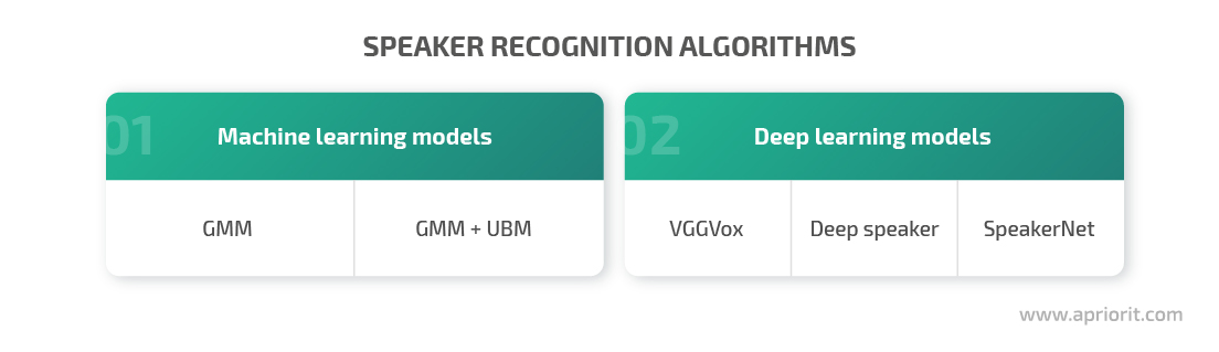
We’ll start with one of the most popular models for processing audio data — the Gaussian Mixture Model.
Gaussian Mixture Model
The Gaussian Mixture Model (GMM) is an unsupervised machine learning model commonly used for solving data clustering and data mining tasks. This model relies on Gaussian distributions, assuming there is a certain number of them, each representing a separate cluster. GMMs tend to group data points from a single distribution together.
Combining a GMM with the MFCC feature extraction technique provides great accuracy when completing speaker recognition tasks. The GMM is trained using the expectation maximization algorithm, which creates gaussian mixtures by updating gaussian means based on the maximum likelihood estimate.
To work with GMM algorithms, you can use the sklearn.mixture package, which helps you learn from and sample different GMMs.
Here’s how you extract features (using the previously described method) and train the GMM using sklearn.mixture:
sample_rate, data = read('denoised_vad_voice.wav')

# extract 40 dimensional MFCC & delta MFCC features
features = extract_features(audio, sr)

gmm = GMM(n_components=16,max_iter=200,covariance_type='diag',n_init=1, init_params='random')
gmm.fit(features) # gmm trainingCombining the Gaussian Mixture Model and Universal Background Model
A GMM is usually trained on speech samples from a particular speaker, distinguishing speech features unique to that person.
When trained on a large set of speech samples, a GMM can learn general speech characteristics and turn into a Universal Background Model (UBM). UBMs are commonly used in biometric verification solutions to represent person-independent speech features.
Combined in a single system, GMM and UBM models can better handle alternative speech they may encounter during speaker recognition, like whispers, slow speech, or fast speech. This applies to both the type and the quality of speech as well as the composition of speakers.
Note that in typical speaker verification tasks, a speaker model can’t be identified directly with the help of the expectation maximization algorithm, as the variety of training data is limited. For this reason, speaker models in speaker verification systems are often trained using the maximum a posteriori (MAP) adaptation, which can estimate a speaker model from UBM.
As for tools, you can use Kaldi — a popular speech recognition toolset for clustering and feature extraction. To integrate its functionality with Python-based workflows, you can go with the Bob.kaldi package that provides pythonic bindings for Kaldi.
Here’s an example of working with Bob.kaldi:
ubm = bob.kaldi.ubm_train(features, r'ubm_vad.h5', num_threads=4, num_gauss=2048, num_iters=100)


# training every gmm using ubm
user_model = bob.kaldi.ubm_enroll(features, ubm)


# scoring using ubm and a specified gmm
bob.kaldi.gmm_score(features, user_model, ubm)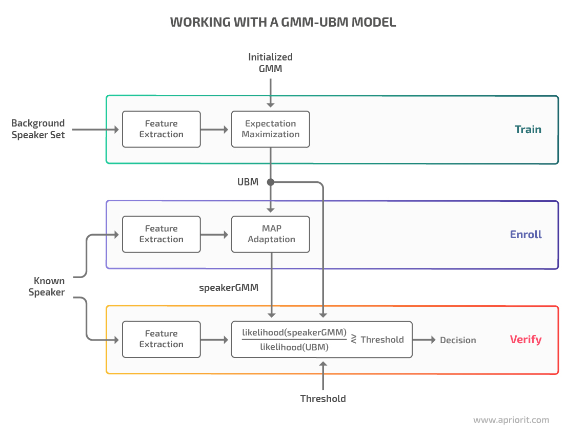
To achieve even higher accuracy, you can try accomplishing speaker recognition tasks with deep learning algorithms. Let’s look at some of the commonly applied DL models in the next section.
Related project
Building AI Text Processing Modules for a Content Management Platform
Find out how Apriorit’s client managed to achieve outstanding user experience, great content management efficiency, and stay competitive in the market thanks to Apriorit’s efforts. Uncover the details of how our team built an efficient AI text processing feature to enhance the client’s platform.

Deep learning models for speaker recognition
When trying to solve speaker recognition problems with deep learning algorithms, you’ll probably need to use a convolutional neural network (CNN). While this type of neural network is widely applied for solving image-related problems, some models were designed specifically for speech processing:
VGGVox is a DL system that can be used for both speaker verification and speaker identification. The network architecture allows you to extract frame-level features from the spectrograms and aggregate them to obtain an audio voice print. To verify a speaker, the system compares voice prints using cosine distance — for similar voice prints, this distance will always be rather small.
To train this model, you need to preprocess your audio data by converting regular audio to the mono format and generating spectrograms out of it. Then you can feed normalized spectrograms to the CNN model in the form of images.
Deep speaker is a Residual CNN–based model for speech processing and recognition. After passing speech features through the network, we get speaker embeddings that are additionally normalized in order to have unit norm.
Just like VGGVox, the system checks the similarity of speakers using the cosine distance method. But unlike VGGVox, Deep speaker computes loss using the triplet loss method. The main idea of this method is to maximize the cosine similarities of two different embeddings of the same speaker while minimizing embeddings of another speaker.
Audio preprocessing for this system includes converting your audio files to 64-dimensional filter bank coefficients and normalizing the results so they have zero mean and unit variance.
SpeakerNet is a neural network that can be used for both speaker verification and speaker identification and can easily be integrated with other deep automatic speech recognition models.
The preprocessing stage for this model also includes generating spectrograms from raw audio and feeding them to the neural network as images.
When working with these models, you can rely on the glob module that helps you find all path names matching a particular pattern. You can also use the malaya_speech library that provides a rich selection of speech processing features.
Here’s what working with these DL models can look like in practice:
# load model
def deep_model(model: str = 'speakernet', quantized: bool = False, **kwargs):
  """
  Load Speaker2Vec model.

  Parameters
  ----------
  model : str, optional (default='speakernet')
      Model architecture supported. Allowed values:

      * ``'vggvox-v1'`` - VGGVox V1, embedding size 1024
      * ``'vggvox-v2'`` - VGGVox V2, embedding size 512
      * ``'deep-speaker'`` - Deep Speaker, embedding size 512
      * ``'speakernet'`` - SpeakerNet, embedding size 7205

  quantized : bool, optional (default=False)
      if True, will load 8-bit quantized model.
      The quantized model isn’t necessarily faster, it totally depends on the machine.

  Returns
  -------
  result : malaya_speech.supervised.classification.load function
  """

model = malaya_speech.speaker_vector.deep_model('speakernet')

from glob import glob

speakers = ['voice_0.wav', 'vocie_1.wav', 'voice_2.wav']

# pipeline
def load_wav(file):
  return malaya_speech.load(file)[0]

p = Pipeline()
frame = p.foreach_map(load_wav).map(model)
r = p.emit(speakers)

# calculate similarity
from scipy.spatial.distance import cdist

1 - cdist(r['speaker-vector'], r['speaker-vector'], metric = 'cosine')However, choosing the right ML or DL model is not enough for building a well-performing speaker recognition system. In the next section, we discuss how setting the right parameters can greatly improve the performance of your machine learning models.
Read also
Navigating AI Image Processing: Use Cases and Tools
Get the most out of artificial intelligence for image processing tasks. In this article, we cover the core stages of this process, common use cases, and helpful tools. Read on to discover the challenges of crafting an AI-based image processing solution and how to address them.

Improving model performance with parameter tuning
There are factors affecting speaker recognition accuracy and the performance of your model. One of these factors is hyperparameters — parameters that a machine learning model can’t learn directly within estimators. These parameters are usually specified manually when developing the ML model.
Setting the appropriate values for hyperparameters can significantly improve your model’s performance. Let’s take a look at ways you can choose the right parameters and cross-validate your model’s performance based on the example of the Scikit-learn library.
Choosing parameters with grid search
Note: To follow through with our examples, you need to install the Scikit-learn library.
There’s no way to know the best values for hyperparameters in advance. Therefore, you need to try all possible combinations to find the optimal values.
One way to train an ML model with different parameters and determine parameters with the best score is by using grid search.
Grid search is implemented using GridSearchCV, available in Scikit-learn’s model_selection package. In this process, the model only uses the parameters specified in the param_grid parameter. GridSearchCV can help you loop through the predefined hyperparameters and fit your estimator to your training set. Once you tune all the parameters, you’ll get a list of the best-fitting hyperparameters.
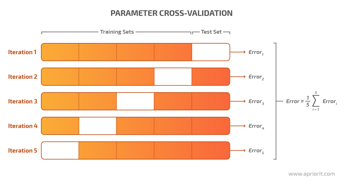
Along with performing grid search, GridSearchCV can perform cross-validation — the process of choosing the best-performing parameters by dividing the training and testing data in different ways.
For example, we can choose an 80/20 data splitting coefficient, meaning we’ll use 80% of data from a chosen dataset for training the model and the remaining 20% for testing the model. Once we decide on the coefficient, the cross-validation technique applies a specified number of combinations to this data to find out the best split.
This is where the pipeline comes into play.
Related project
Developing an Advanced AI Language Tutor for an Educational Service
Explore the insights of building an AI-powered language learning tutor for our client’s e-learning product. Discover how the Apriorit team helped the client become more competitive by introducing interactive language learning and improving user experience.

Cross-validating a model with pipelines
A pipeline is used to assemble several steps that can be cross-validated while setting different parameters for a model.
There are must-have methods for pipelines:
-
- The fit method allows you to learn from data
- The transform or predict method processes the data and generates a prediction
Scikit-learn’s pipeline class is useful for encapsulating multiple transformers alongside an estimator into one object so you need to call critical methods like fit and predict only once.
We can get the pipeline class from the sklearn.pipeline module.
You can chain transformers and estimators into a sequence that functions as a single cohesive unit using Scikit-learn’s pipeline constructor. For example, if your model involves feature selection, standardization, and regression, you can encapsulate three corresponding classes using the pipeline module.
And if you are using custom functions to transform data at the preprocessing and feature extraction stages, you might need to write custom transfer and classifier classes to incorporate these actions into your pipeline.
Here’s an example of a custom transformer class:
import numpy as np
import warnings
from python_speech_features import mfcc, delta
from sklearn import preprocessing
from sklearn.utils.validation import check_is_fitted

warnings.filterwarnings('ignore')
from sklearn.base import BaseEstimator, TransformerMixinAnd this is what a CustomTransformer(TransformerMixin, BaseEstimator) class would look like:
def __init__(self, winlen=0.020,preemph=0.95,numcep=20,nfft=1024,ceplifter=15,highfreq=6000,nfilt=55,appendEnergy=False):
self.winlen = winlen
self.preemph = preemph
self.numcep = numcep
self.nfft = nfft
self.ceplifter = ceplifter
self.highfreq = highfreq
self.nfilt = nfilt
self.appendEnergy = appendEnergy
def transform(self, x):
""" A reference implementation of a transform function.
Parameters
----------
x : {array-like, sparse-matrix}, shape (n_samples, n_features)
The input samples.
Returns
-------
X_transformed : array, shape (n_samples, n_features)
The array containing the element-wise square roots of the values
in ``X``.
"""
# Check is fit has been called
check_is_fitted(self, 'n_features_')
# Check that the input is of the same shape as the one passed
# during fit.
if x.shape[1] != self.n_features_:
raise ValueError('Shape of input is different from what was seen'
'in `fit`')
return self.signal_to_mfcc(x)
def fit(self, x, y=None):
"""A reference implementation of a fitting function for a transformer.
Parameters
----------
x : {array-like, sparse matrix}, shape (n_samples, n_features)
The training input samples.
y : None
There is no need of a target in a transformer, yet the pipeline API
requires this parameter.
Returns
-------
self : object
Returns self.
"""
self.n_features_ = x.shape[1]
return selfIf you need a custom classifier class, this is what it might look like:
import numpy as np
import warnings
from python_speech_features import mfcc, delta
from sklearn import preprocessing
from sklearn.utils.validation import check_is_fitted

warnings.filterwarnings('ignore')
from sklearn.base import BaseEstimator, TransformerMixinYou might also need to create additional methods to load data and extract features and sample rates.
Here’s how you can create a load data method:
def load_data(folder):
  x, y = [], []

  for voice_sample in list(glob.glob(rf'./{folder}/id*/id*')):
      voice_sample_file_name = os.path.basename(voice_sample)
      voice_class, _ = voice_sample_file_name.split("_")

      features = read_wav(voice_sample)

      x.append(features)
      y.append(voice_class)

return np.array(x, dtype=tuple), np.array(y)And here’s what the code of a method to extract features and sample rate can look like:
def read_wav(fname):
  fs, signal = wavfile.read(fname)
  if len(signal.shape) != 1:
      signal = signal[:,0]
return fs, signalThe parameters for the param_grid module should be specified using documentation for the defined method. It’s important to mention the list of different values or the range of values.
If you’re using binary outcomes (true or false), you need to define only two values. When working with categorical values, you need to create a list of all possible string values.
Here’s an example of how to determine the best-fitting parameters using grid search and a pipeline:
x, y = load_data('test')


# creating pipeline of transformer and classifier
pipe = Pipeline([('scaler', CustomTransformer()), ('svc', CustomClassifier())])


# creating the parameters grid
param_grid = {
    'scaler__appendEnergy': [True, False],
    'scaler__winlen': [0.020, 0.025, 0.015, 0.01],
    'scaler__preemph': [0.95, 0.97, 1, 0.90, 0.5, 0.1],
    'scaler__numcep': [20, 13, 16],
    'scaler__nfft': [1024, 1200, 512],
    'scaler__ceplifter': [15, 22, 0],
    'scaler__highfreq': [6000],
    'scaler__nfilt':[55, 0, 22],
    'svc__n_components': [2 * i for i in range(0, 12, 1)],
    'svc__max_iter': list(range(50, 400, 50)),
    'svc__covariance_type': ['full', 'tied', 'diag', 'spherical'],
    'svc__n_init': list(range(1, 4, 1)),
    'svc__init_params': ['kmeans', 'random']
}
search = GridSearchCV(pipe, param_grid, n_jobs=-1)
# searching for appropriate parameters
search.fit(x, y)To illustrate how different parameters can affect the performance of an ML model, we tested the previously discussed models on different datasets. Go to the next section to see the results of these tests.
Read also
AI Speech Emotion Recognition for Cybersecurity: Use Cases and Limitations
Elevate your software with advanced features for speech emotion recognition (SER). Read the full article to find out how SER works, where to use it, and what concerns and nuances to be aware of.
Evaluating the impact of parameter tuning
We tested the performance of two machine learning models: a combination of GMM and MFCC and the GMM-UBM model. For better test result accuracy, we compared the performance of these models on two datasets:
1. LibriSpeech — This dataset is a collection of around 1,000 hours of audiobook recordings. The training data is split into three sets: two containing “clean” speech (100 hours and 360 hours) and one containing 500 hours of “other” speech, which is considered more challenging for an ML model to process. The test data is also split into two categories: clean and other.
Here’s the structure of the LibriSpeech dataset:
.- train-clean-100/
              |
              .- 19/
                  |
                  .- 198/
                  | |
                  | .- 19-198.trans.txt
                  | |
                  | .- 19-198-0001.flac
                  | |
                  | .- 14-208-0002.flac
                  | |
                  | ...
                  |
                  .- 227/
| ...2. VoxCeleb1 — This is one of two audio-visual VoxCeleb datasets formed from YouTube interviews with celebrities. In contrast to LibriSpeech, this dataset doesn’t have many clean speech samples, as most interviews were recorded in noisy environments.
The dataset includes recordings of 1251 celebrities, with a separate file for each person. Each file has subfolders with WAV audio files, and each subfolder depicts the YouTube video that was used to create the speech samples.
Here’s the structure of this dataset:
.- vox1-dev-wav/
|          |
|          .- wav/
|              |
|              .- id10001/
|              |   |
|              |   .- 1zcIwhmdeo4/
|              |   |      |
|              |   ...    .- 00001.wav
|              |
|              .- id10002/
|                    |
|                    ...
|First, we tested a simple GMM-MFCC model trained on the LibriSpeech dataset. The results are the following:
Table 1 – Testing a GMM-MFCC model on the LibriSpeech dataset
| Number of users | Level of accuracy |
| 100 users | 98.0% accuracy |
| 1000 users | 95.8% accuracy |
As this dataset contains clean speech samples, the results for LibriSpeech are always good, whether we use a GMM-MFCC, GMM-UBM, or any other machine learning model. For this reason, all other tests will be focused on the VoxCeleb dataset, which is a lot more challenging for a machine learning model to process.
Let’s start with the results of testing a GMM-MFCC model using the VoxCeleb dataset:
Table 2 – Testing a GMM-MFCC model on the VoxCeleb dataset
| Number of users | Level of accuracy |
| 100 users | 84.8% accuracy |
| 1000 users | 72.1% accuracy |
As you can see, the accuracy of our model decreased significantly, especially when applied to a larger number of users.
Now let’s take a look at the results of testing a GMM-UBM model trained on the VoxCeleb dataset:
Table 3 – Testing a GMM-UBM model on the VoxCeleb dataset
| Number of users | Level of accuracy |
| 100 users | 92% accuracy |
| 1000 users | 84% accuracy |
This model proved to be more accurate than the GMM-MFCC model.
We can also see how changing the parameters of a model affects its performance. For this example, we tested the MFCC model and its delta and delta + double delta versions on 100 users:
Table 4 – Testing the influence of parameter changes
| Parameters | MFCC | MFCC + delta | MFCC + delta + double delta |
| numcep=13 | 81.6% accuracy | 77.6% accuracy | 80.3% accuracy |
| numcep=20 | 87.6% accuracy | 87.0% / 89.0% accuracy | 83.0% accuracy |
The numcep value represents the number of cepstrums to return. As you can see, the higher the numcep, the more accurate the results our models show.
And as for the deep learning models mentioned in this article, they showed the following results when trained on the VoxCeleb dataset and tested on 100 users:
Table 5 – Testing DL models on the VoxCeleb dataset
| Model | Level of accuracy |
| SpeakerNet | 97% accuracy |
| VGGVox | 96% accuracy |
| Deep speaker | 75% accuracy |
As you can see, the performance of different ML and DL methods depends greatly on both the parameters specified for your model and the dataset you use to train it. So before making a final choice on the ML or DL model for your speaker recognition project, it would be best to test several models on different datasets to find the best-performing combination.
Conclusion
Speech recognition is the core element of complex speaker recognition solutions and is commonly implemented with the help of ML algorithms and deep neural networks. Depending on the complexity of the task at hand, you can combine different speaker recognition technologies, algorithms, and tools to improve the performance of your speech processing system. You can also use them for generative AI development and other types of projects.
When in doubt, consult a professional! Apriorit’s AI development team will gladly assist you with choosing the right set of parameters, tools, datasets, and models for your AI project.
Need assistance with AI & ML fueled software?
Focus on your project’s bigger picture by leaving the engineering matters to Apriorit’s qualified developers!
Have a question?
Ask our expert!
R&D Delivery Manager